
POTENTIAL PROBLEMS
35
is given
by
u* —
—UVLV
(c)
The source formulation gives
u= au*dr- bu*dQ
(d)
Equation (d) can be applied
at
points
x = 0
and
x =
1,
to
obtain,
"o
=
o"i(isin l) +
i x
sin
x dx = 0
u
i
—
σ
ο(ι^
η
l) + i
x s
^
n
(1 —^)dx
= 0
Jo
This system gives,
1 cosl
4
<7
0
=
^—r-1,
*!=-—--1
(
f
)
sin
1
sin 1
Note that these two values for the sources are the same as the q
0
and
q
x
of
Example
1.7.
2.4 MATRIX FORMULATION
We will now explain how the boundary element techniques described
in Sections 2.2 and 2.3 can be interpreted
in
matrix form. The direct
case given by relationship (2.23) will be considered in detail. This case
is more general than equations (2.35) and (2.36) which can also
be
rendered into matrix form.
Consider equation (2.23) specialised
for
the boundary points and
without
the
term
in p for
simplicity (the case with
p is
considered
later),
i.e.
K+
uq*
dr
=
qu*dr
(2.41)
Assume
for
simplicity that
the
body
is
two dimensional and
its
boundary
is
divided into
N
'segments'
or
'boundary' elements,
as
shown
in
Figure 2.4.
The
points where
the
unknown values
are
36 POTENTIAL PROBLEMS
Figure 2.4 Boundary elements: (a) constant;
(b) linear; (c) quadratic
(b)
considered are called 'nodes' and taken to be in the middle of each
segment for the so-called 'constant' elements (Figure 2.4(a)). These
are going to be the only elements considered in this section, but in the
next chapter we will also discuss the case of linear elements (i.e.
elements for which the nodes are at the intersection between elements
as shown in Figure 2.4(b)) and curved elements such as the quadratic
ones shown in Figure 2.4(c). For the latter case an extra mid-element
node is required and the elements are called quadratic.
For the constant element case the boundary is discretised into N
elements, of which N
i
are assumed to belong to Γ
ί
andN
2
tor
2
.The
values of u and q are assumed to be constant on each element and
equal to the values at the mid-node of the element. Note that on each
POTENTIAL PROBLEMS
37
element
one
of
the two
variables
(u or q)
is
known.
Equation (2.41)
can
be
discretised
for a
given point
T
before
applying
any
boundary conditions,
as
follows,
N
r N r
fa*
Σ uq*dr=
X
qu*dr (2.42)
j =
i Jrj j
=
l
Jr,.
Note that
for
this type
of
element
the
boundary
is
always 'smooth'
hence
the
multiplier
of
w,
is j.
Γ
}
is
the
boundary
of
element
'/.
Formula (2.42) applies for a particular node
T. The u
}
and
q
}
values
can
be
taken
out of the
integrals
as
they
are
assumed
to be
constant
over each element. This gives,
ΐ".
+
Σ
(
[
9*
dr
)»J =
Σ
(J
"*
dr
J
(2·
43
)
The integrals
j
q*
άΓ
relate
the
V
node with
the
segment
'/
over
which
the
integral
is
carried
out. We
shall call these integrals
Η^. The
integrals
on the
right-hand side
are
of
the
type
J
u*
άΓ and
will
be
called
G
tJ
.
Hence
we can
write (2.43)
as,
±11,+
Σ
#0";=
Σ
Giili
(
2
·
44
)
j
= i j
=
i
The integrals
can
easily
be
calculated analytically
but for
higher-
order elements they become more difficult
to
evaluate
and
they
are
usually evaluated numerically.
We can rewrite equation (2.44)
for
each i node under consideration.
Let
us now
call
j Η^ when
i
Φ
j
[Hij
+
i
when
i =7
Hence equation (2.44)
can now be
written
as,
Σ H
u
uj= Σ Gijlj
(
2
·
4
*)
7=1
7=1
The whole
set
of equations can also
be
expressed
in
matrix form as,
H
U
=
G
Q
(2.47)
Note that
N
x
values
of
u
and
N
2
values of q are known
on Γ,
hence
38 POTENTIAL PROBLEMS
one has a set of only N unknows in formula (2.47) which can be
reordered according with the unknown under consideration. We can
pass all unknowns to the left-hand side and write,
AX= F
(2.48)
where X is the vector of unknown w's and g's.
Equation (2.48) can now be solved and we then know all the
u's
and
g's values on the boundary. Once this is done we can calculate the
values of w's and q's at any interior point using equation (2.17), i.e.
u
t
= qu*dr- uq*dr (2.49)
The w's can be obtained directly from (2.49) by discretising it as
follows,
"1= Σ 4jGij- Σ "flu (2.50)
j =
i j = i
The values of internal fluxes can be calculated by differentiating
(2.49),
which gives (see Figure 2.5) for a point i
du
du
q^r-άΓ
q——di
dy
u—-dr
i
r
ex
Γ
Sq*
fr
dy
(2.51)
0X interior &
x
boundary
Figure 2.5 Derivatives of
a
function at the interior point 'Γ
POTENTIAL PROBLEMS 39
EVALUATION OF INTEGRALS
The integrals H
0
and G
u
can be calculated using the simple Gauss
quadrature rule (four points for the two-dimensional case) for all
points, except the one corresponding to the node under consideration.
For this integral it is recommended to use higher-order integration
rules or a special logarithmic formula which will be described later on.
For the particular case of constant elements, however, the H
ti
and G
u
integrals can be easily computed analytically. The H
H
term for
instance is identically zero, for fundamental solutions with no
Γ dependence, i.e.
H
it
=
q*dr =
du*
dr
dr dn*
άΓ = 0
(2.52)
This is because n and r are orthogonal over the element.
The G
u
integral can be calculated analytically as follows,
G,.
=
f
w
*dr =
i- j
In
0 W (2.53)
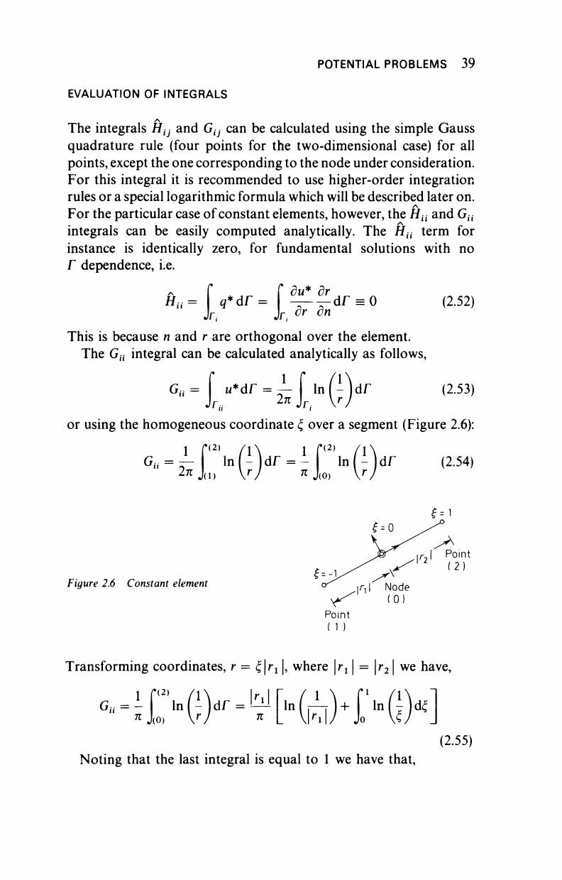
or using the homogeneous coordinate ξ over a segment (Figure 2.6):
ο
»
=
έίΓ'"0>
Γ
%-Ι>(Ο
αΓ
,251)
Figure 2.6 Constant element
f=-i
Transforming coordinates, r = ξτ
ι
,
where 1^ | ^
j/-
2
1
we have,
G
u
= -
π
(2)
i(0)
'"Oh^KräH'
1
"©«]
(2.55)
Noting that the last integral is equal to 1 we have that,
..................Content has been hidden....................
You can't read the all page of ebook, please click here login for view all page.