
4 Fundamental
Solutions
4.1 INTRODUCTION
We have seen, in Chapter 2, a few examples of fundamental solutions
for a number of simple differential equations. Before we go on to look
at more complicated problems it is essential that we
first
consider their
physical significance and study their mathematical properties.
We shall start by introducing the Dirac delta function as a sum of
eigenfunctions, and then go on to consider some methods of finding
the explicit form of fundamental solutions for some commonly
occurring problems.
At the end of the chapter will be found a table of the fundamental
solutions for a selection of differential equations (Table 4.1).
4.2 EIGENFUNCTIONS AND THE DIRAC DELTA FUNCTION
Consider a medium in which we have a physical property represented
by the function u which may be a function of space and time. If we
know the governing equation for u and this equation is linear (non-
linear problems will be dealt with in Chapter 6) we can write this
equation as
J5?(II) = 0 (4.1)
throughout the medium which we shall for the moment consider to be
finite in extent.
Here if is a linear differential operator, for which we have
80
FUNDAMENTAL SOLUTIONS 81
Χ(*φ
1
+βφ
2
) = *Χ{φ
1
) + βΧ(φ
2
) (4.2)
where
φ
γ
and φ
2
are any two
functions with sufficient continuity
properties
to
make
^{φι) and
&
?
(φ
2
)
meaningful,
and a and β are
constants.
The eigenfunctions
φ
η
corresponding
to
S£
are
defined
by
&(Φη)
=
ΚΦη
(4.3)
where
λ
η
is a
constant called
the
eigenvalue corresponding
to the
eigenfunction
φ
η
.
The form
of the
eigenfunctions will depend
on the
coordinate
system used. For rectangular Cartesian coordinates we can choose the
eigenfunctions to be the harmonic functions cos
(nx),
sin
(nx),
cos
(ny
etc.,
or using complex notation
e
±inx
.
The eigenvalues
λ
η
are then just
polynomials involving powers
of
Ή'
and 'in' for an
equation with
constant coefficients.
1
It
is
usual
to
choose our eigenfunctions
to
be
a
complete set, in
the
sense that
for any
function
u a
number
N can be
found such that
N
<
ε (4.4)
where
ε is any
small number
and a„ are
constants.
Here we have used
'| |
11'
to
denote the norm of a function defined
by
''-" -
71-·
άΩ
(4.5)
where
the
integration
is
over
all the
variables
in u on the
problem
region, Ω and
Λ
denotes complex conjugation. Equation (4.4) means
that we can expand any sufficiently continuous function
u
in terms
of
a series
of
eigenfunctions
to any
desired degree
of
accuracy,
i.e.
«=
lim
(Σ**Φ*)
<
4
·
6
)
N
-►
oo n = 0 /
In this chapter
we
shall
use the
notation
<
Μ)1;
>
Ω
= uvdQ
(4.7)
(u,v}
r
= uvdr
(4.8)
82 FUNDAMENTAL SOLUTIONS
to represent integration of the two functions
u
and
v
over the region Ω
and boundary
Γ
respectively. The expression
<
u,
v
>
Ω
which will be
a
number,
is
referred
to as the
'scalar product'
of
u
and v.
The norm
of
a function
u may now be
written
IMI
=
V<
w
>">«
(4.9)
Given a complete set of eigenfunctions we may form an orthonormal
set which
has the
property that
<Φ^Φ
η
>
Ω
=
δ
ηιη
(4.10)
where S
mn
is the
Krönecker delta defined
by
~ ίθ
ifm^n
Ö
mn=L
:c (
4
-U)
We may now define the Dirac delta function on the region in terms
of
our complete orthonormal
set for
this region,
by
00
δ
Ω
(Χ-ξ)=
Σ
Φη(*)Φη(ξ) (4-12)
«
= 0
where
3c
and
ξ
are two points in space. Hereafter we shall refer to ξ
as
the 'source' point
and
3c
as the
observation point.
For
the
case
^
=
έ
6Χρ
(
ίη
τ)
(the eigenfunctions corresponding
to the
one-dimensional Laplace
equation over the interval
—
a
to
a) the delta function for this region
will
be
represented
by:
at
«
1
v
(
ϊηπχ
(
mn
S
1 £ (\
40*
By the nature
of
the expansion we have assumed that this function
is
periodic with period
2a,
so if we plot this function in the range
-
a
to a
we will have ignored 'image' functions repeating outside the region at
distances
of
2na.
FUNDAMENTAL SOLUTIONS 83
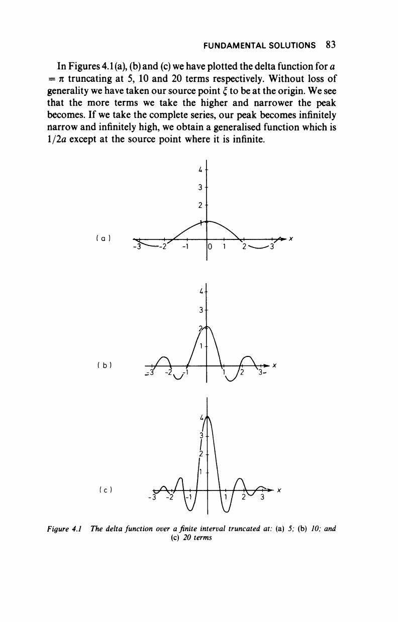
In Figures
4.1
(a),
(b)
and (c) we have plotted the delta function for a
= π truncating at 5, 10 and 20 terms respectively. Without loss of
generality we have taken our source point ξ to be at the origin. We see
that the more terms we take the higher and narrower the peak
becomes. If we take the complete series, our peak becomes infinitely
narrow and infinitely high, we obtain a generalised function which is
l/2a except at the source point where it is infinite.
(a)
Figure 4.1 The delta function over a finite interval truncated at: (a) 5; (b) 10; and
(c) 20 terms
84 FUNDAMENTAL SOLUTIONS
We can see that as a 'forcing function' on the right-hand side of an
equation this would give for the solution the field due to a series of
sources separated by twice our normalisation range.
We shall illustrate the definitions given above with a simple
example.
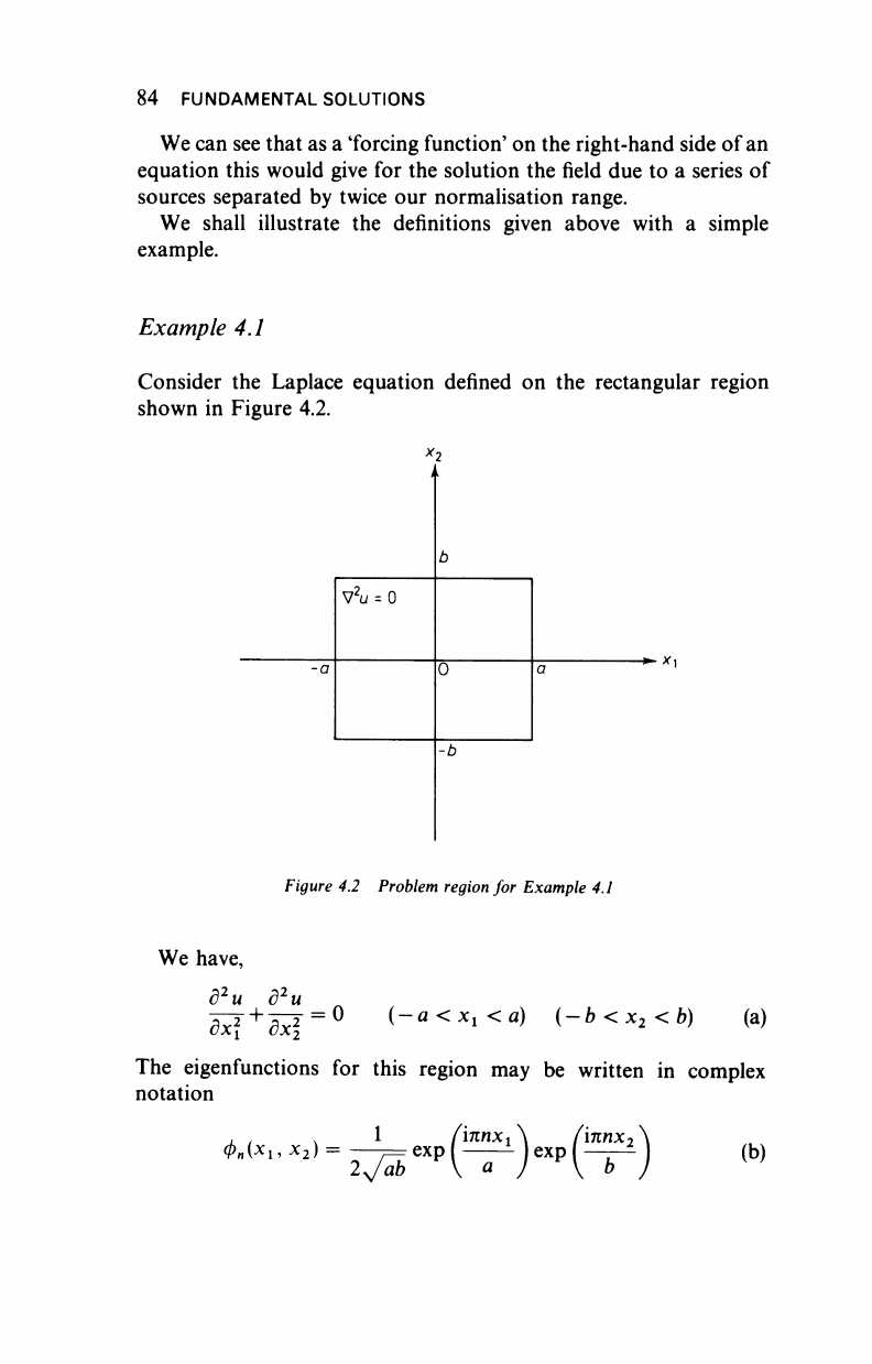
Example 4.1
Consider the Laplace equation defined on the rectangular region
shown in Figure 4.2.
V
2
L/
= 0
*2
-►*i
-b
Figure 4.2 Problem
region
for Example 4.1
We have,
d
2
u d
2
u
^y +
^2-
= ° (-fl<Xi <a)
(-b<x
2
<b)
(a)
The eigenfunctions for this region may be written in complex
notation
JL
t ^ 1
ίπηχ
1
i
nx
2
Φη(Χι,
*i) = —^exp exp'
2 Jab a
] v
(b)
..................Content has been hidden....................
You can't read the all page of ebook, please click here login for view all page.