
APPROXIMATE METHODS 3
and,
βι =
u — ü
Φ 0 on /
ε
2
= q
—
q Φ 0 oni
2
Our aim is now to make this error as small as possible over the
domain and on the boundary. In order to do so the errors can be
distributed and the way in which this distribution is carried out
produces different types of weighted residual techniques.
1.2 WEIGHTED RESIDUAL TECHNIQUES
The simplest of these techniques starts by exactly satisfying the
boundary conditions (i.e. ε
ι
= ε
2
= 0) and distributing the error
according with a weighting function w. This function is such that it
identically satisfies the homogeneous boundary conditions and can be
written as,
>ν
= 0
1
ΐΑΐ+02</'2+03</'3+ ..· (1.8)
The
ij/i
are members of a set of known linearly independent functions
and ßi are arbitrary coefficients. We will call them w
t
when they are
arbitrary nodal coefficients.
The distribution of the error function ε can now be carried out by
multiplying it by the weighting function w and integrating over the
domain, i.e.
ewdQ= (V
2
u)wdQ = 0 (1.9)
In this way the error is distributed in accordance with the functions in
w. Note that because the
/?,
coefficients are arbitrary, (1.9) can also be
written as,
(V
2
i#
t
dß = 0 for i = 1, 2, . . ., n (1.10)
h
Classical finite difference techniques for instance can be interpreted
as a special case of equation (1.9) for which the weighting functions
are Dirac delta functions, and the ß
t
are nodal arbitrary coefficients
(w,),
such that,
w = w
l
6
1
4-νν
2
^
2
+
νν
3^3 + .·. (1-11)
4 APPROXIMATE METHODS
The Dirac delta function is a generalised function which can be
defined as the limit of a normal function such as
■im
Sin[
*
(
*-*'
)]
=*(*-*,) (1.12)
yv-oo n(x-Xi)
In the limit this function is zero at every point except where the
argument is zero where it is infinite (i.e. at x = x,). Thus it represents a
point singularity at the 'source' point x
t
.
The delta function has the property that
Γ °° CXi + a
ö(x-x
i
)dx= (5(x-x;)dx=l (1.13)
J -
oo
Jx, - a
for a any positive number.
We also have that for any function/(x) (continuous at x
f
) we can
write
r oo ΛΧ,- + a
f(x)S(x-
Xi
)dx= f(x)ö(x-x
i
)dx=f(x
i
) (1.14)
J -
oo
Jx,-ü
Where it is not necessary to represent the arguments of the functions
explicitly in the analysis we shall use the shorthand notation putting
ö(x-x
i
) = ö
i
and (1.15)
f(Xi)=fi
for simplicity. Where it is important to include the arguments for
clarity of explanation we shall use the full notation writing x and x,
explicitly.
The approximating functions are given by
u = η
1
φ
ί
+ η
2
φ
2
+ ιι
3
φ
3
+ . . . (1.16)
(The φί are localised second-order polynomials taken over the
subdomain surrounding the node for the central difference scheme.)
Substituting (1.16) into (1.9) produces the following equation at
each node T:
e<
5
i
.dO =
ei
= 0 (1.17)
Ω
The above presentation gives the same numerical results as the
central finite difference scheme for quadratic approximating func-
tions.
The procedure is however, more general as it allows us equally
APPROXIMATE METHODS 5
well to use other types of φ
{
functions. Furthermore the basic ideas
can be generalised. Using curvilinear coordinates these generali-
sations give rise to the 'cell collocation' method.
1
Basically this is a
subregion collocation technique as shown in Example 1.1.
Example 1.1
Consider the equation
dx
where x varies from 0 to 1 with boundary conditions
u(0)
= u(l) = 0 (b)
Cell
2
+
w
+ x = 0 xe[0, 1] (a)
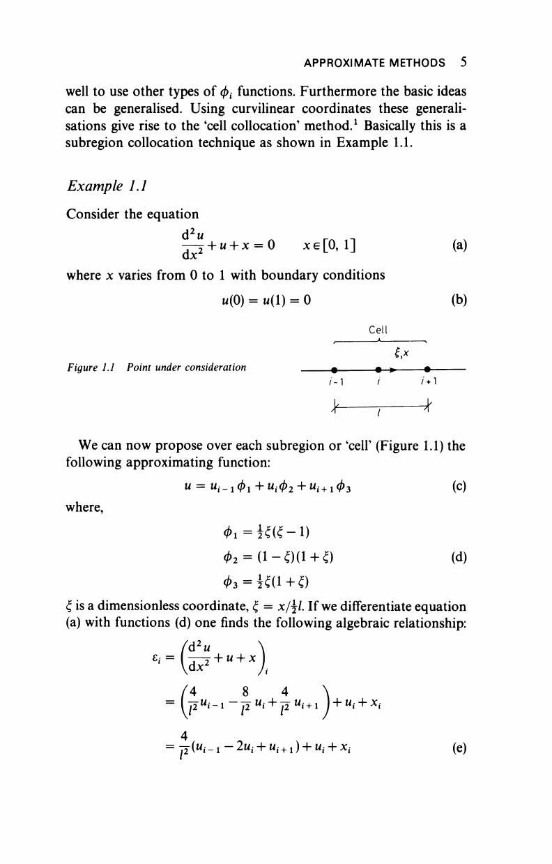
Figure 1.1 Point under consideration * +
>
%—
/-1 / /♦!
* ; *
We can now propose over each subregion or 'cell' (Figure 1.1) the
following approximating function:
" = "i-101+"i02 + "i+103 (C)
where,
φ
2
= (1-ξ)(ί + ξ) (d)
ζ is a dimensionless coordinate, ξ = x/L If
we
differentiate equation
(a) with functions (d) one finds the following algebraic relationship:
(d
2
u
/4 8 4
= j2
U
i-l--J2
U
i + ]2
U
i+l
J
+
U
i +
X
i
4
= 72("i-i-
2
»i +
M
i+i) +
M
i + -
x
i (e)
6 APPROXIMATE METHODS
This
ε^
is made equal to zero at i according to equation (1.11), which
gave the same result as central finite differences, for this particular
case.
METHOD OF MOMENTS
Equation (1.9) can be used to generate a wide variety of weighted
residual techniques such as the method of moments, the original
Galerkin method, collocation, subregions, etc.
The method of moments consists in taking moments of the error
function. For instance for a one-dimensional problem this implies
taking moments of ε with respect to the following function:
1,
x, x
2
, . . . (1.18)
These are the φ
(
functions of equation (1.8). Hence we can write a
weighting function such that,
χν
= β
1
ψ
1
+β
2
ψ
2
+
β
3
ψ
3
+
...
= β
1
1+β
2
χ +
β
3
χ
2
+
...
(L19)
The method is illustrated with the following example.
Example 1.2
Assume to have the same equation and boundary conditions as seen in
Example 1.1. The error function is
d
2
u
ε = —
T
+
u
+ x (a)
ax
z
We can propose an approximating function that satisfies the boun-
dary conditions and such as,
u
=
α
ι</>ι + a
2
02+ . . . = ajx(l -x) + a
2
x
2
(l -x) + ... (b)
Note that the φ
ί
,φ
2
, ··· functions satisfy the homogeneous
boundary conditions at x = 0 and x = 1. The a, coefficients are
unknown and are not directly associated with nodal values of the u
functions as we have not defined any nodes over the domain. The
error function for two a, coefficients results
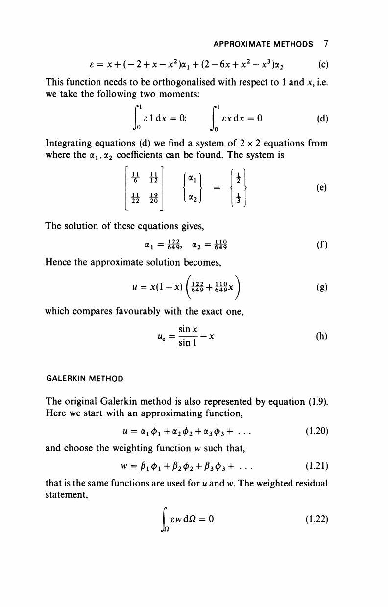
APPROXIMATE METHODS 7
ε = x +
(
—
2 + x
—
x
2
)oc
1
+ (2
—
6x + x
2
—
x
3
)<x
2
(c)
This function needs to be orthogonalised with respect to 1 and x, i.e.
we take the following two moments:
ε
1
dx = 0; εχ dx = 0 (d)
Jo
Integrating equations (d) we find a system of 2 x 2 equations from
where the α
1?
α
2
coefficients can be found. The system is
-
11
6
11
22
_
-
11
12
19
20
_
The solution of these equations gives,
a
l — 649»
a
2 — 649
Hence the approximate solution becomes,
u =
x(i-x)(m+mx
which compares favourably with the exact one,
sinx
it* = ——-
—
x
sin
1
(e)
(f)
(g)
(h)
GALERKIN METHOD
The original Galerkin method is also represented by equation (1.9).
Here we start with an approximating function,
u = α
1
φ
1
+α
2
0
2
+ α303+ · · ·
and choose the weighting function w such that,
(1.20)
(1.21)
that is the same functions are used for
u
and w. The weighted residual
statement,
h
ewdQ = 0
(1.22)
..................Content has been hidden....................
You can't read the all page of ebook, please click here login for view all page.