
114 FUNDAMENTAL SOLUTIONS
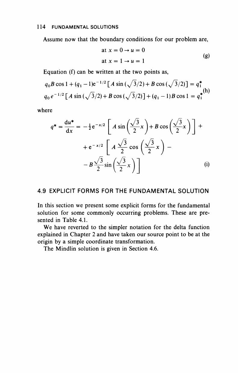
Assume now that the boundary conditions for our problem are,
atx = 0->w = 0
atx=l->w=l
Equation (f) can be written at the two points as,
q
0
B cos
1
+ (q
x
- l)e"
1/2
[A sin (^3/2) + B cos (^3/2)] = q*
r- r- (h)
^
0
e"
1/2
[i4sin(
N
/3/2) + Bcos(
N
/3/2)] + (g
1
-l)Bcosl = q[
where
+
q* =
-j—
= -^e
x/2
A sin l^z-x
)
+ £cos(^—x
dx * V 2 / V 2
_|_
e
x/2 A jv__
COS
I
->L_
x
) _
[^cos(-^x)
RV3 . Λ/3
ß
T-
sin
V
x
(i)
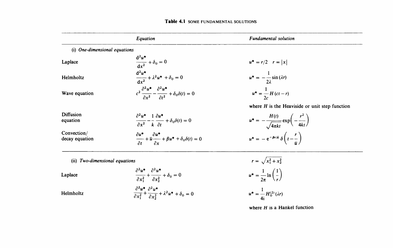
4.9 EXPLICIT FORMS FOR THE FUNDAMENTAL SOLUTION
In this section we present some explicit forms for the fundamental
solution for some commonly occurring problems. These are pre-
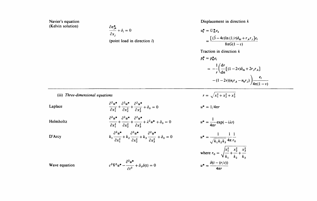
sented in Table 4.1.
We have reverted to the simpler notation for the delta function
explained in Chapter 2 and have taken our source point to be at the
origin by a simple coordinate transformation.
The Mindlin solution is given in Section 4.6.
Table
4.1 SOME FUNDAMENTAL SOLUTIONS
Equation
Fundamental solution
(i)
One-dimensional
equations
Laplace
Helmholtz
Wave equation
Diffusion
equation
Convection/
decay equation
d
2
u*
d^
d
2
u*
+
<5
0
= 0
+ /l
2
u*
+<5
0
= 0
dx
2
d
2
u* d
2
u*
dx
2
dt
2
d
2
u* 1 du*
dx
2
k dt
du*
du*
+
ü
+ ßu* +δ
0
δ(ή = 0
dt dx
u* = r/2 r = x
1
u* = sin (Ar)
2λ
1
u*
=— H(ct-r)
2c
where H is the Heaviside or unit step function
(■
H(t)
u* = exp
yJAnkt
u* =
-Q-
ßrlü
δ
■-)
4ktJ
(ii)
Two-dimensional
equations
Laplace
Helmholtz
d
2
u* d
2
u*
d
2
u* d
2
u*
u*=—ln(-)
2π
/
u*=—H
{
0
2)
(Xr)
4i
where /i is a Hankel function

Table 4.1 (continued)
Equation
Fundamental solution
(ii) Two-dimensional equations
D'Arcy
Wave equation
Plate
equation
Reduced
plate
equation
d
2
u* d
2
u*
dx dx
(orthotropic case)
(d
2
u*
d
2
u*
c
2
[
dx
2
i* d
2
u* d
2
u
+
c5
0
<5(t)
= 0
*+<5
0
<5(t) = 0
V
4
= (V
2
)
2
in two dimensions
k
p
= ω/μ
(V
4
-/c>*+<5
0
= 0
1 1 /1
u*=
—
In
1—1
Jk,k
2
2π Vr
o'
fx] xiy-
where r
0
= I 1 I
H(ct-r)
2nc(c
2
t
2
-r
2
>ral sine f
f
00
sini;
Si(")=- di;
J
u
V
Hit)
4πμ 4μί
Sj is the integral sine function
1 / 2i
— H^(k
p
r)
K
0
(k
p
\ki π
8i/c
2
where K
0
is an elliptic function
Navier's equation
(Kelvin solution)
dXj
(point load in direction /)
Displacement in direction k
"* = Vf
k
e
k
_[(3-4i;)ln(l/r)^ +
r
ik
r
<
>
i
8πσ(1-ι;)
Traction in direction k
liar
= — — [(l-2v)<5
/k
+ 2r
(i
r,
fc
]
r άη
-(l-2v)(n
l
r
t
-
4π(1-ν)
(iii)
Three-dimensional
equations
d
2
u* d
2
u* d
2
u*
Laplace
Helmholtz
D'Arcy
Wave equation
d
2
u* d
2
u* d
2
u*
Γ + Γ + - + ^
2
"* +
<5
0
= 0
dx
2
dx
2
dx
2
d
2
u* d
2
u* d
2
u*
d
2
u*
c
2
V
2
u*--—+^(t)
= 0
dt
2
r= Jx + x + x
u* = 1/4πΓ
1
u* = exp(-Ur)
4nr
1 1 1
V^Ms
4
*
1
"«
X
l
X
2
X
3
where r
0
= / 1 H
k k
2
k$
S(t-(r/c))
4nr
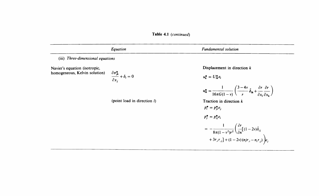
Table 4.1 (continued)
Equation
Fundamental solution
(iii) Three-dimensional equations
Navier's equation (isotropic,
homogeneous, Kelvin solution) daj
k
3X:
+
<5,
= 0
(point load in direction /)
Displacement in direction k
1 /3-4v . dr dr
(1-v) V r
'*
+
ä^ä^/
16nG(l
Traction in direction k
P*
= Pfa
+ 3r
|
.r
J
] + (l-2v)(n7>
|
.-ii
|
.r
J
.)j^
J
·
..................Content has been hidden....................
You can't read the all page of ebook, please click here login for view all page.