
128 ELASTOSTATICS
5.5 MATRIX FORMULATION
We can now work with matrices instead of using the indicial notation.
In order to do so we can define u as the displacement, p as the traction
and b as the body force vectors, such that
(5.34)
At a point i these displacements are called u
1
. In addition we can
define the following two matrices:
u =
«1
"2
«3
·. P =
Pi
Pi
.Ps.
, b =
<
*i ;
^2
Λ j
u =
«Tl
«21
«?1
«12
«?2
"32
«ί
3
"
«23
«Ϊ3
, P* =
"pTi
P*I
_P!I
ph
P*2
P*2
phi
P*3
P33J
(5.35)
where the u
lk
and p
lk
are the displacements and forces in the k
directions due to a unit force at the point
1
under consideration, acting
in the / direction.
Let us
first
write formula (5.27) before any boundary conditions are
applied, i.e.
cM+ pr
k
u
k
dr= ur
kPk
dr+ uf
k
b
k
aQ (5.36)
Jr Jr Jß
This equation can now be expressed in matrix form as follows,
c
f
Ui+
p*udr= u*pdr+ u*bdß (5.37)
This formulation is valid for a point i. Note that p*, u* and b are
known and c
t
will soon be determined. The unknowns are the values
of u and p over the boundary.
BOUNDARY ELEMENTS
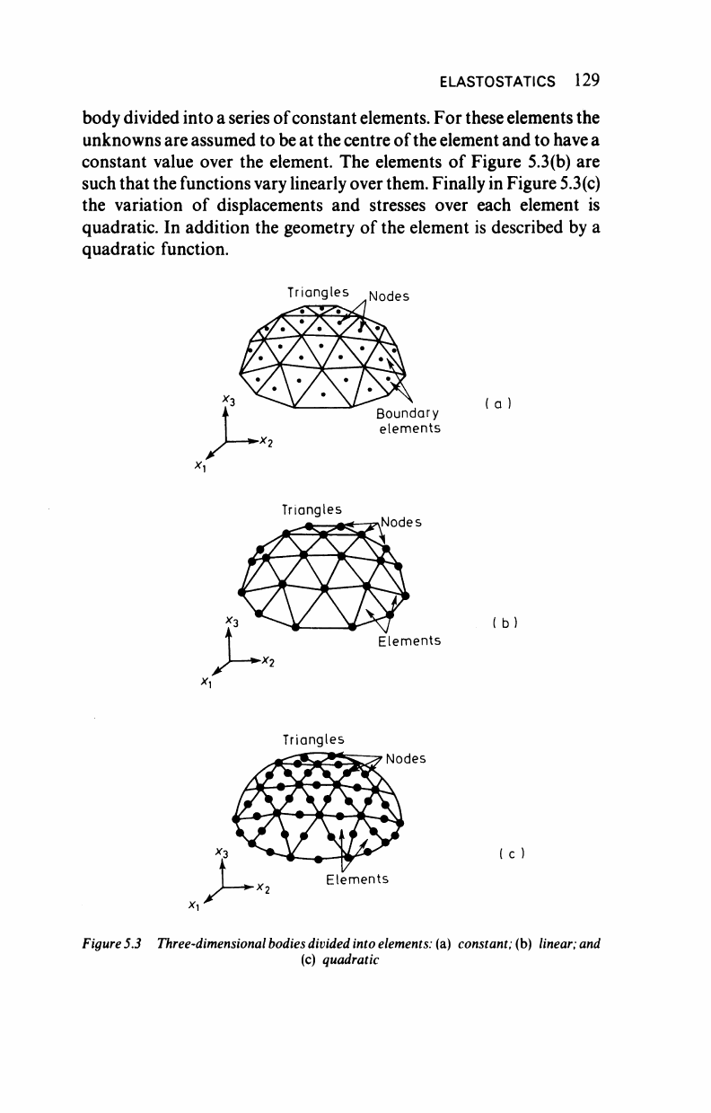
We will now assume that the boundary is divided into elements. These
boundary elements can be constant, linear, quadratic or higher order
and they can be triangles or quadrilaterals. Figure
5.3(a)
shows the
ELASTOSTATICS 129
body divided into a series of constant elements. For these elements the
unknowns are assumed to be at the centre of the element and to have a
constant value over the element. The elements of Figure
5.3(b)
are
such that the functions vary linearly over them. Finally in Figure
5.3(c)
the variation of displacements and stresses over each element is
quadratic. In addition the geometry of the element is described by a
quadratic function.
Triangles
Nodes
Boundary
elements
Triangles
Nodes
b)
Elements
Triangles
Nodes
( c )
Elements
Figure
5.3
Three-dimensional
bodies divided into
elements:
(a)
constant;
(b)
linear;
and
(c) quadratic
130 ELASTOSTATICS
Over each element the functions for u and p can be approximated
using the following interpolation functions:
U = 0
T
U
n
=
Φ
Ί
p=
Ψ
τ
ρ
η
=
Φ
1
Φ
Ί
u
n
(5.38)
P
n
(5.39)
Note that the functions for u and p are generally different. For
consistence it may be better to take the functions for p of one order
less than those for u. The interpolation functions are the ones
discussed in Chapter 3. u
n
, p
n
are the nodal displacements and
tractions.
We can substitute the above functions into (5.37) and obtain the
following equation for the point i:
c,u,+ Σ (| P*4>
T
drju
n
= Σ (f
u*y
T
drV
M Λ
+
Σ U*
j=*
JO™
+
bdß (5.40)
where the summation from j = 1 to N indicates summation over the
N elements on the surface and Γ, is the surface of the) element. The
summation from; = 1 to M is carried out over the internal cells and
Q
m
is the volume of each of them.
The integrals in equation (5.40) are usually solved numerically and
the functions Ψ and φ are expressed in some of the homogeneous
system of coordinates described in Chapter
3.
The integrals need then
to be written in terms of the homogeneous system, to be called ξ, η.
Hence
dr = (absolute value of |G|) άξάη
(5.41)
where G has been defined previously.
Due to the difficulties in integrating equation (5.40) it is usual to
ELASTOSTATICS 131
employ a numerical integration scheme. Hence formula (5.40)
becomes,
Ί"ι+
Σ ( Σ |0|νν
Γ
(ρ*φ
τ
(ξ^))Λυ
η
j=
1
=l /
=
Σ ( Σ
|ο|νν
Ρ
(υ*ψ
τ
(ξ
)>
/)))ρ"
+ Σ ί Σ
Mk(u*b)
r
)
j =
1
r =
1
/ j =
1
r =
1
/
(5.42)
J
is the
Jacobian
for
the
three-dimensional transformation,
and w
r
are
the numerical integration weighting coefficients.
Note that (5.42) gives a set of equations for node i which can be
written as,
CjUi
+ ^fi«...
fi„...
fi
ir
] <
u,
t
"r
J
(5.43)
= [9ii 9i2 · · · 9Ü · · · 9ι>]
Pi
P
2
P,
v
P
V
+ b
f
where u
7
and p^ are the unknowns at nodes
j.
fi
0
and g
0
are the
interaction coefficients relating node i. with all the nodes on the
surface of the body. Note that with the exception of constants
elements, more than one element will contribute to the fi
0
and g
0
submatrices. (They
are 3
x
3
for the three-dimensional case and 2x2
for two dimensions.)
132 ELASTOSTATICS
SYSTEM EQUATIONS
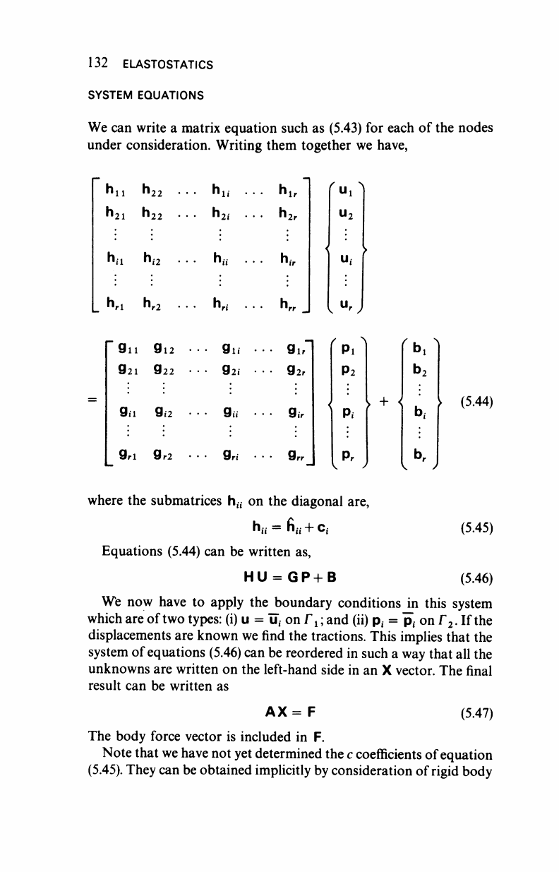
We can write a matrix equation such as (5.43) for each of the nodes
under consideration. Writing them together we have,
h
n
h
22
h
1(
h
21
h
22
· · · h
2l
. .
h
a
h
i2
h
u
h
rl
h
r2
h
ri
9u 9i2 ··· 9ii ·
921 922 · · · 92/ ·
9ii 9.2 . · · 9u ·
9rl 9r2
h
lr
h
2r
9r
Ό
u
f
K
J I
U
r
9 ι,Ί
92r
9ir
9rr_
<
f
Pi
Pi
Pi
►
+ <
fbil
b
2
b,
> (5.44)
b
r
where the submatrices h
u
on the diagonal are,
h
fl
= h
u
+ c,
Equations (5.44) can be written as,
HU=GP+B
(5.45)
(5.46)
We now have to apply the boundary conditions in this system
which are of
two
types: (i) u =
"u,
on Γ
χ
; and (ii) p
f
= p) on Γ
2
. If the
displacements are known we find the tractions. This implies that the
system of equations (5.46) can be reordered in such a way that all the
unknowns are written on the left-hand side in an X vector. The final
result can be written as
AX= F
(5.47)
The body force vector is included in F.
Note that we have not yet determined the c coefficients of equation
(5.45).
They can be obtained implicitly by consideration of
rigid
body
..................Content has been hidden....................
You can't read the all page of ebook, please click here login for view all page.