
62 HIGHER-ORDER ELEMENTS
3.3 QUADRATIC AND HIGHER-ORDER ELEMENTS
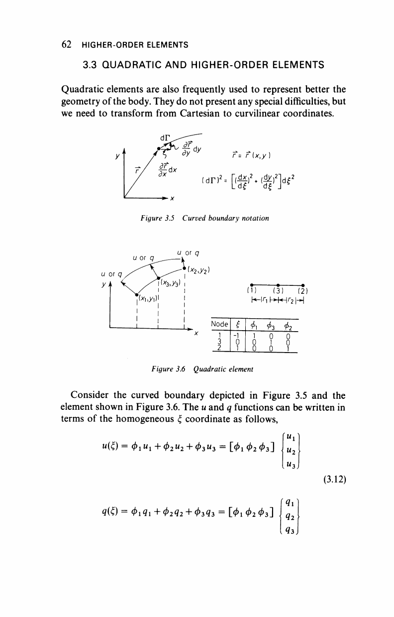
Quadratic elements are also frequently used to represent better the
geometry of the body. They do not present any special difficulties, but
we need to transform from Cartesian to curvilinear coordinates.
dr,2
=['f
2
*'t
2
K
Figure 3.5 Curved boundary notation
u or q
(*2>y2)
(1) (3) (2)
Node
1
3
2
ΊΓ
-1
0
1
4>y
1
0
0
<t>2
0
1
0
Φ?
0
0
1
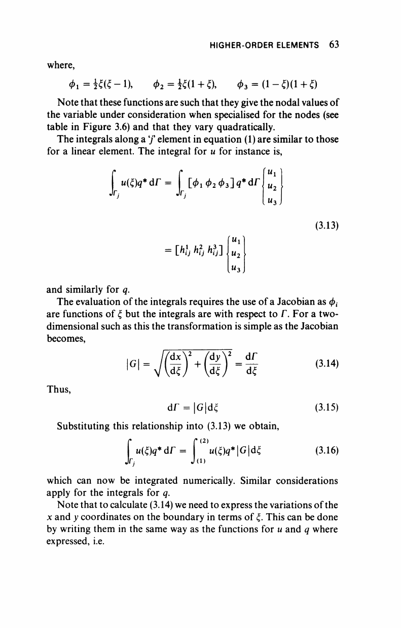
Figure 3.6 Quadratic element
Consider the curved boundary depicted in Figure 3.5 and the
element shown in Figure 3.6. The
u
and q functions can be written in
terms of the homogeneous ξ coordinate as follows,
U(£)= (^Ui + φ
2
U
2
+
(/)
3
U
3
=
[</>!
φ
2
</>
3
]
*3)
(3.12)
,4i
<!(£)=
<Ml +</>2^2 +
</>3<?3
= Ol Φΐ Φζ] q
2
43
HIGHER-ORDER ELEMENTS 63
where,
Φι=*«ί-1λ
tf>2 = i£(i
+
a
03 = (i-Od
+
0
Note that these functions are such that they give the nodal values of
the variable under consideration when specialised for the nodes (see
table in Figure 3.6) and that they vary quadratically.
The integrals along a'/ element in equation (1) are similar to those
for a linear element. The integral for u for instance is,
[
u(Qq*dr
=[ίΦι ΦζΦζ^άΑ
(3.13)
=
[W·?;]
and similarly for q.
The evaluation of the integrals requires the use of
a
Jacobian as φ
{
are functions of ξ but the integrals are with respect to Γ. For a two-
dimensional such as this the transformation is simple as the Jacobian
becomes,
G =
dx
+
dT
d£
Thus,
df = |G|d£
Substituting this relationship into (3.13) we obtain,
[uü)q*ar= ί
(2)
η(ξ^*�άξ
Jfj J(l)
(3.14)
(3.15)
(3.16)
which can now be integrated numerically. Similar considerations
apply for the integrals for q.
Note that to calculate (3.14) we need to express the variations of the
x and y coordinates on the boundary in terms of
ξ.
This can be done
by writing them in the same way as the functions for u and q where
expressed, i.e.
64 HIGHER-ORDER ELEMENTS
X = φ
1
Χ
χ
+
φ
2
Χ
2
+ </>
3
*3
(3.17)
x,·,^
are the coordinates of
a
node referred to the global system (see
Figure 3.5).
It will be shown that in order to be able to reproduce the constant
potential type conditions, the order of the
u
function has to be at least
the same as the function for x and
u
used to describe the geometry of
the body.
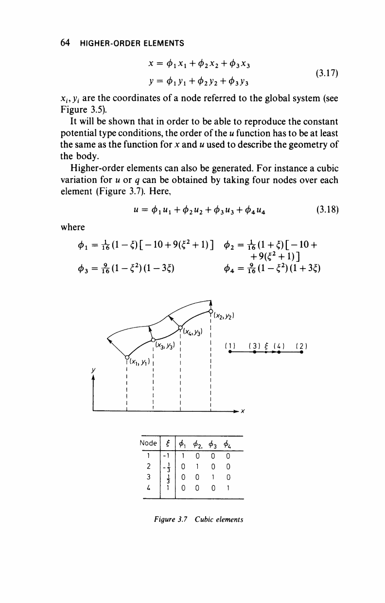
Higher-order elements can also be generated. For instance a cubic
variation for u or q can be obtained by taking four nodes over each
element (Figure 3.7). Here,
U = φ
1
«
1
+(/)2"2 + Φ3"3 + 04"4
(3.18)
where
φ
1
=&(1-ξ)ί-10
+
9(ξ
2
+
1)-
φ
2
= &(1
+
ξ)[-10 +
+ 9(ξ
2
+
1)~
φ
3
= &(1-ξ
2
)(1-3ξ) φ
Α
= ±(1-ξ
2
)(1
+
3ζ)
13) ξ U) (2)
Node
1
2
3
L
ξ
-1
1
-7
1
7
1
^
1
0
0
0
Φι.
0
1
0
0
4>2 Φί*
0 0
0 0
1 0
0 1
Figure
3.7
Cubic elements
..................Content has been hidden....................
You can't read the all page of ebook, please click here login for view all page.