
FUNDAMENTAL SOLUTIONS
85
as
δ
2
φ 6
2
φ
η
π
2
η
2
( 1
~eÄ
+
-äÄ
=
~Yj7bV
2+
b
i
r
(c)
The nth eigenvalue
is
thus given
by:
These eigenfunctions are orthonormal
as
<4>m> Φη>Ω=
I I
</>m<Mx
2
dXl
r
+
ίπηχ
2
1
C*
f* /
+
/πηχΛ
b
—
ιπηιχ,χ
—
mx
2
t
x exp
I I
exp
I I
dx
2
d.Xi
=
4^Jl
eXP
(~
i,t(m
"
M)
^)
dXl><
x exp
( —
in(m
—
n)-^
)dx
2
fl form
= n)
:
(0
for
m
^
n J
The eigenfunctions form
a
complete
set as the
expansion
in (4.6)
becomes:
1
"
V
°°
m
V
°°
(χπηχΛ (inmx
2
iC
^
u{x
l9
x
2
)
= —-=
Σ Σ
a
nw
exp I—— exp
I——I
(f)
2Jabn=-oom=-oo
a
/ ° /
which
is the
complex form
of
the double Fourier expansion
of
the
function
u
over
the
rectangular region.
Note. The expansion
(f)
assumes that
u is a
periodic function
of χ
λ
and
x
2
with periods 2a and 2fc respectively. This does not concern
us
here
as we are
only interested
in
solving
the
equation inside
the
rectangle.
86 FUNDAMENTAL SOLUTIONS
In this region we can write our Dirac delta function:
SQ(X-T)
= <M*i - £i)<M*2 - ξ
2
)
1
£ (
inn
<
*
Λ
=
4^
n
i
oo
exp^-(x
1
-^)jx
xexpl + — (χ
2
-ξ
2
)
(g)
where our source point is (ξ
ί9
ξ
2
) and our observation point is
(x
1
,x
2
).
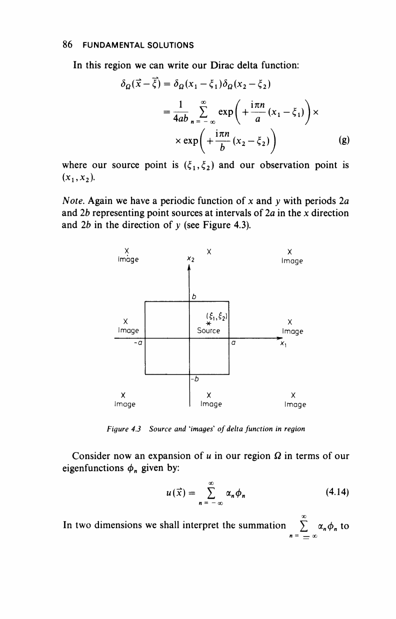
Note. Again we have a periodic function of x and y with periods 2a
and 2b representing point sources at intervals of
2a
in the x direction
and 2b in the direction of y (see Figure 4.3).
x
Image
X
Image
X
Image
X
Image
Source
X
Image
-b
X
Image
X
Image
Figure 4.3 Source and
'images'
of delta function in region
Consider now an expansion of u in our region Ω in terms of our
eigenfunctions φ
η
given by:
«(?)= Σ *ηΦη (
4
·14)
n = - oo
00
In two dimensions we shall interpret the summation £
<χ
η
φ
η
to
n = — oo
FUNDAMENTAL SOLUTIONS 87
oo 00
mean the double summation ]Γ Σ
α
η η
Φη
χ
η
2
where η = (n
l9
η
χ
=
—
αο
η
2
=
—
οο
η
2
).
For simplicity we shall omit the vector sign off the suffices.
Now consider
<H(X
15
χ
2
),(5
Ω
(χ-£)>
β(ί)
(d)
for our case this becomes
η(χ
1
,χ
2
)δ
Ω
(χ-ξ)άχ
ί
άχ
2
J-a J-b
=
ü££
w(xi
'
x2)exp
(-v
(xi
-
i
>
)
)
x
xexpf - — (χ
2
-ξ
2
) jdx!dx
2
1 £ Γ / ίπ<
= —7= 2.
ex
P + ε
χ
Ρ
ιπηξ
2
1
b
2^/äb
. . ϊπηχ
ί
( innx
2
, Ί
w(xi,x
2
)exp( —- ]exp( ^ Jdx^Xi (e)
i/(Xi .XT )exD
I
i-"fi
b
a
J
b
The integral appearing here is again the form of the Fourier
coefficient a„ in the expansion of u, so we may write (e) as
- - 1 £ l ίηηξΛ
<ι/(χ
1
,χ
2
),(5
Ω
(χ-0>
Ω(
ί
)
= --7= Σ
ex
P(
+
—7~"J
X
v
lyjab
n = o
V " /
χ
ε
χρ(
+
^)α„ (f)
but this is just the Fourier expansion of
ϋ(ξ
ί9
ζ
2
) hence we have
demonstrated a special case of equation (4.18), i.e.
<u(x
1
, x
2
),<M*-<f)>ß(x)= ußuti) (g)
88 FUNDAMENTAL SOLUTIONS
Multiplying
by
4>
m
and integrating over
Ω we
obtain:
=
-
ao
/
00
= Σ *η(ΦηιΦτη^Ω
= Σ
*n?>nm
=
<*m
(4.15)
n
=
—
oo
<*m
=
<Ml,0
m
>fl (4.16)
an expression
for
our expansion coefficients
a
m
.
iVoie. For the case φ
γη
=
(2n)~
l
&
nmx
(the eigenfunctions for the one-
dimensional Laplace equation, over
the
interval
—
π
to π) the
left-
hand side corresponds
to a
finite Fourier transform
of
u giving
the
Fourier coefficient
cc
m
.
Now consider
the
expression
<u(x),S
a
(x-t)y
Q
(4.17)
we may write both terms
as
expansions
in
terms
of
our
<f>„:
Σ
*.ΦΛΧ),
Σ
<l>m(x)$m(Z)
m
=
0
0(x)
00 00
= Σ
α
» Σ #.»(£)< Φη(χ)>Φιη(χ) >
Ω(χ)
n
=
0
m
=
0
00 00
Hence
=
Σ
α
* Σ
^m(i)^nm
n
=
0
m
=
0
oo
Σ
«ηΦΛΪ)
= «(f)
<u(x),<M*-£)V, = "(£) (4.18)
We have
now
derived
the
selective property
of a
delta function
which
we
shall use extensively
in
what follows.
..................Content has been hidden....................
You can't read the all page of ebook, please click here login for view all page.