
8 APPROXIMATE METHODS
can now be written as
εφ
ί
άΩ = 0 i=l, 2, ... (1.23)
It is also common in Galerkin method to write the
w
function as Au,
i.e.
w = Au
where
Au = Αα
1
φ
ί
+ Ja
2
$2 + ^
a
-3$3+ · · · (1-24)
and
AoLi
= /?
f
.
This representation is sometimes preferred to indicate that
w
can be
identified with a variation or virtual quantity (such as virtual
displacements or velocities). Expression (1.24) also indicates that the
same functions are used for
u
as for
Au.
This.property is important as
it produces symmetry in the expressions as we will see in Example 1.3.
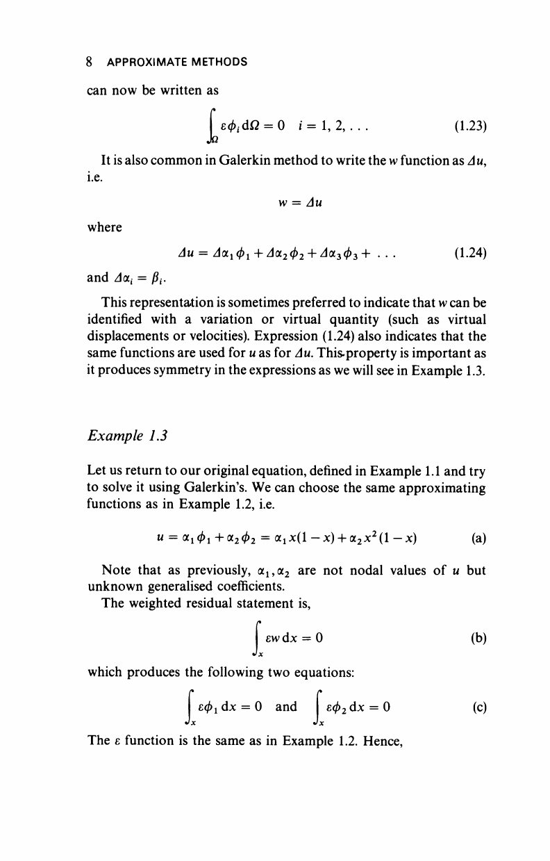
Example 1.3
Let us return to our original equation, defined in Example 1.1 and try
to solve it using Galerkin's. We can choose the same approximating
functions as in Example 1.2, i.e.
u = (χ
ι
φ
ι
+<χ
2
φ
2
= ajx(l -χ) +
α
2
χ
2
(1
-x) (a)
Note that as previously,
α
1?
α
2
are not nodal values of u but
unknown generalised coefficients.
The weighted residual statement is,
ί
ενν
dx = 0 (b)
c
which produces the following two equations:
I
εφ
ι
dx = 0 and
εφ
2
dx = 0 (c)
The ε function is the same as in Example 1.2. Hence,
APPROXIMATE METHODS 9
ί
[x
+ (-
2
+ x -
χ
2
)α
χ
+
(2
-
6x
+
x
2
-
x
3
)a
2
]
[x(l
-
x)]
dx
= 0
(d)
[x
+ (-2 +
x-x
2
)
ai
+
(2-6x
+
x
2
-x
3
)a
2
] [x
2
(l-x)]dx
= 0
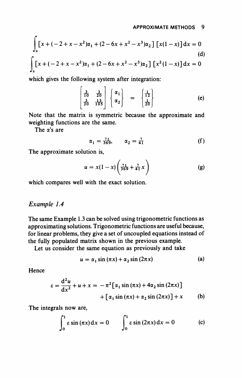
which gives the following system after integration:
ί
_2_
10
3
20
A
13
T0~5
1*1
(e)
Note that the matrix is symmetric because the approximate and
weighting functions are the same.
The a's are
a
l — 369»
The approximate solution is,
OLy
=;
n
= x(l-x)hf& + Ä*J
(f)
(g)
which compares well with the exact solution.
Example 1.4
The same Example 1.3 can be solved using trigonometric functions as
approximating solutions. Trigonometric functions are useful because,
for linear problems, they give a set of uncoupled equations instead of
the fully populated matrix shown in the previous example.
Let us consider the same equation as previously and take
Hence
u =
OL
X
sin (πχ) + α
2
sin (2πχ)
ε = -j-y +
u
+ x = - π
2
[α
χ
sin (πχ) + 4α
2
sin (2πχ)]
d^u
dx
2
+ [ocj sin (πχ)
4-
α
2
sin (2πχ)] + χ
esin(Äx)dx = 0 ε sir
Jo
Jo
The integrals now are,
εύη(πχ)ά
:
sin (2πχ) dx = 0
(a)
(b)
(c)
..................Content has been hidden....................
You can't read the all page of ebook, please click here login for view all page.