
From an operational intelligence standpoint, it is interesting to understand how many visitors we have to our online store and how many of these people actually purchase something. For example, if we have 1,000 people visiting a day but only 10 people actually purchase something, this might indicate something is not quite right. Perhaps, the prices of our products are too high, or the site might be difficult to use and thus need a redesign. This information can also be used to indicate peak purchasing times.
In this first recipe, we will leverage summary indexing to understand how many sessions we have per hour versus how many actual completed purchase transactions there have been. We will plot these over a line graph going back the last 24 hours.
To step through this recipe, you will need a running Splunk Enterprise server, with the sample data loaded from Chapter 1, Play Time – Getting Data In. You should be familiar with navigating through the Splunk user interface and using the Splunk search language.
Follow these steps to leverage summary indexing in calculating an hourly count of sessions versus the completed transactions:
- Log in to your Splunk server.
- Select the Operational Intelligence application.
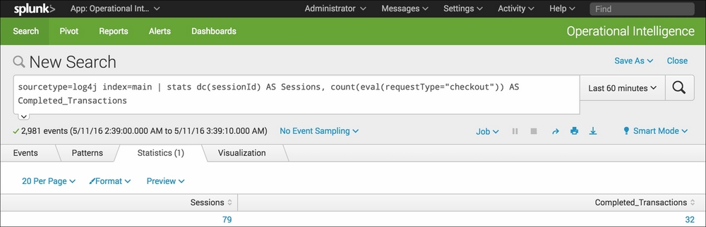
- From the search bar, enter the following search and select to run over Last 60 minutes:
sourcetype=log4j index=main | stats dc(sessionId) AS Sessions, count(eval(requestType="checkout")) AS Completed_Transactions
- Click on the Save As dropdown and select Report from the list:
- In the pop-up box that gets displayed, enter
cp09_sessions_transactions_summaryas the title of the report and select No in the Time Range Picker field; then click on Save:
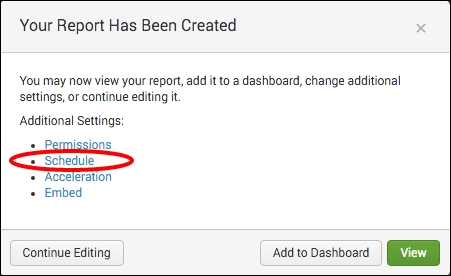
- On the next screen, click on Schedule from the list of Additional Settings:
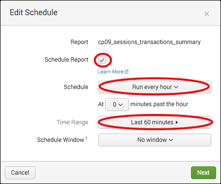
- Select the Schedule Report checkbox, Run every hour in the Schedule field, and a time range of Last 60 minutes. Click on Next, and then simply click on Save on the next screen:
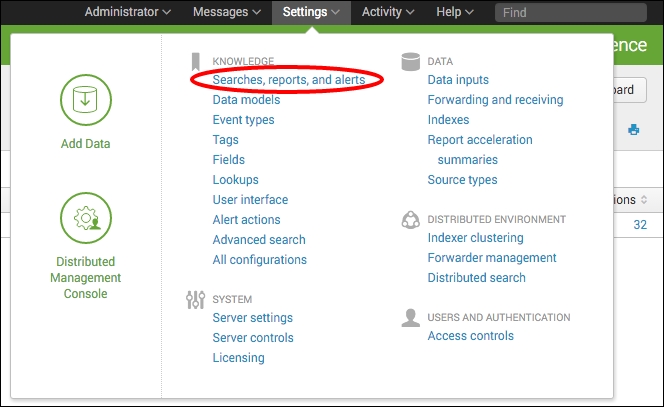
- In order to activate summary indexing on the report that you just saved, you will need to edit the search manually. Click on the Settings menu at the top-right and select Searches, reports, and alerts:
- A list of all the saved searches will be displayed. Locate the search named
cp09_sessions_transactions_summaryand click on it to edit it. - The search editor screen will be displayed. Scroll down to the very bottom—Summary indexing section—and select the Enable checkbox. Ensure that the default summary index called summary is selected, and then click on Save:

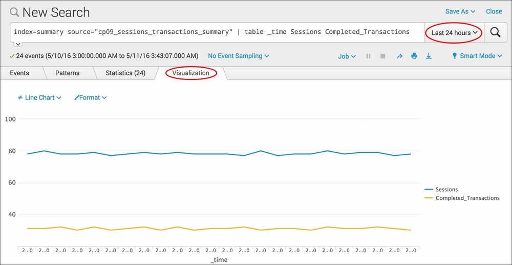
- The search is now scheduled to run every hour, and the results are scheduled to be written to a summary index named summary. After 24 hours have passed, run the following search from the search bar in the Operational Intelligence application, with a time range set to Last 24 hours:
index=summary source="cp09_sessions_transactions_summary" | table _time Sessions Completed_Transactions
- The search will complete very fast and list 24 events, one for each hour. Select the Visualization tab to see the data presented as a line chart representing sessions versus completed transactions:
- Let's save this as a report, and then add the report to a dashboard panel. Click on the Save As dropdown and select Report.
- Enter
cp09_sessions_vs_transactionsin the Title field of the report, and ensure that the Content field is set to Line Chart. Then click on Save: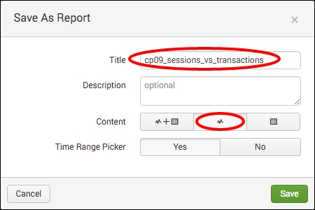
- On the next screen, click on the Add to Dashboard button.
- In the pop-up box that appears, select New to add a new dashboard and give it a title of
Session and Purchase Trends. Ensure that the permissions are set to Shared in App and give the panel you are adding a title ofHourly Sessions vs Completed Transactions. Ensure that the panel is powered by Report and the Panel Content is set to Line Chart. Then click on Save to create the new dashboard with the line-chart panel: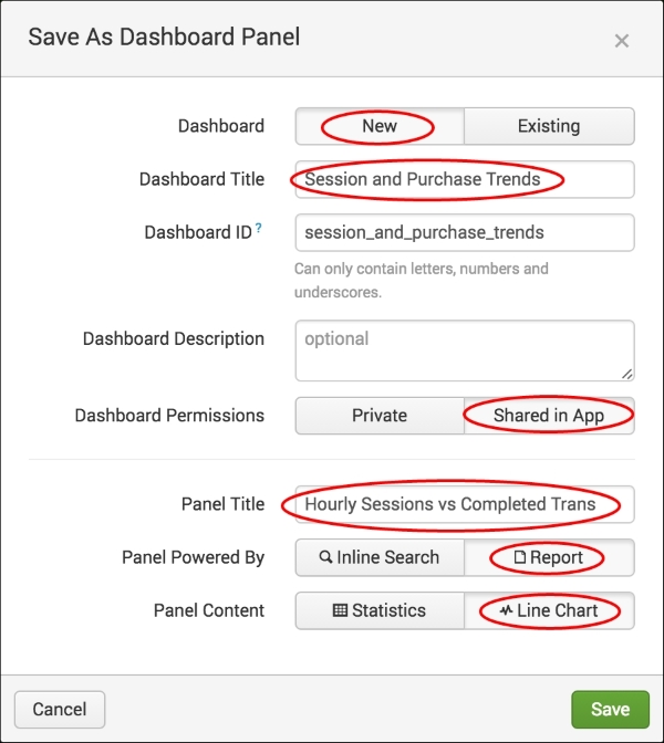
In this recipe, you created a scheduled search that will take hourly snapshots, counting the number of unique sessions and the sessions that resulted in completed purchase transactions. Every hour, the search runs, a single line item with two values is created, and the results are written to a summary index named summary. Returning to the search 24 hours later, you are able to run a report on the summary index to instantly see the activity over the past day in terms of sessions versus purchases. There will be 24 events in the summary, one for each hour. Reporting off the summary data is a lot more efficient and faster than attempting to search across the raw data. If you wait longer, say 30 days, then you can run the report again and plot the results across an entire month. This information might then be able to provide predictive insights into the sales forecast for the next month.
There were two searches that you used for this recipe. The first search was used to generate the summary data and ran hourly. The second search was used to search and report against the summary data directly. Let's break down each search piece by piece:
Search 1 – summary index generating search
|
Search fragment |
Description |
|---|---|
sourcetype=log4j index=main |
We first select to search the application data in the main index over the past hour. |
| stats dc(sessionId) AS Sessions, count(eval(requestType="checkout")) AS Completed_Transactions |
Using the |
Search 2 – reporting off the summary index
index=summary source="cp09_sessions_transactions_summary" |
We first select to search the summary index. Then, within this index, we look for data with a source of |
| table _time Sessions Completed_Transactions |
We tabulate the data by time, number of sessions, and number of completed transactions. |
Tip
If you search the summary data directly, you will notice that Splunk gives the summary data a sourcetype field value of stash by default. However, the source field value for the data will be the name of the saved search. Therefore, searching by source rather than sourcetype is likely to be your preferred approach.
As you can see, summary indexing is a great way to shrink down our raw dataset to just the valuable data that we need to report on. The raw dataset still exists, so we can create many summaries off the same data if we want to do so.
In this recipe, the summary-generating search was set to run hourly and look back over the past hour. This results in a single event being generated per hour and written to the summary. If more granularity is required, the search can be set to run every 15 minutes; look back over the past 15 minutes and four events per hour will be generated. As the search is now only looking back over the past 15 minutes instead of the past hour, it will likely execute faster as there is less data to search over. For some data sources, generating the summary index data more frequently over smaller chunks of time can be more efficient.
Care needs to be taken when creating summary index generating searches to avoid both gaps in your summary and overlaps in the data being searched.
For example, you schedule a summary index generating search to run every 5 minutes and look back over the past 5 minutes, but the search actually takes 10 minutes to run. This will result in the search not executing again until its previous run is complete, which means it will run every 10 minutes, but only look back over the past 5 minutes. Therefore, there will be data gaps in your summary. This can be avoided by ensuring that adequate search testing is performed before scheduling the search.
In another example, you schedule a summary index generating search to run every 5 minutes and look back over the past 10 minutes. This will result in the search looking back over 5 minutes of data that the previous run also looked back over. Therefore, there will be data overlaps in your summary. This can be avoided by ensuring that there are no overlaps in time when scheduling the search.
Additionally, gaps can occur if you take the search head down for an extended period of time and then bring it back up. Backfilling can be used to fill in past gaps in the data, and this is discussed in the next recipe.