Hayek (1937, 1945) was the first to point out that competitive market prices carry useful information and, like the invisible hand, coordinate economic activity and allocation of scarce resources. In the absence of the right market structure though, the invisible hand of the price system is not potent enough to ensure efficient resource allocations, for example, Pareto-efficient allocations when no one can get better off without making someone else worse off.

The notion of complete markets first appeared in the groundbreaking Arrow-Debreu model of general equilibrium as a simple market structure supporting Pareto efficiency (Arrow, 1951; Debreu, 1951; Arrow and Debreu, 1954). In fact, in complete markets every competitive equilibrium is Pareto-optimal (by the First Welfare Theorem). The original Arrow-Debreu model featured a static setting with production, exchange, and consumption all taking place at once. Without a time dimension, the original model had no room for time uncertainty and financial assets, and market completeness was defined by frictionless exchange of state goods rather than state securities.

Apples and oranges are examples of state goods. It would have been inefficient and cumbersome for both producers and consumers if apples and oranges had been sold only as a package and not individually. Yet corporate bonds have always traded as packages consisting of an interest-rate component and a credit component. Only in recent years, with the advent of interest-rate derivatives and credit derivatives, has it become possible to unbundle corporate bonds by separating credit from interest rates. Whether building a portfolio of physical goods or financial securities, a complete set of basic building elements, such as state goods and state securities, helps to achieve better portfolio allocations.

Subsequent versions of the Arrow-Debreu model included a time interval between 0 and 1, time uncertainty and financial assets (Arrow, 1964; Debreu, 1959). At time 0, the agents first assign subjective probabilities to the states of the world at time 1 and next make allocations to time-0 consumption and to financial assets designed to finance time-1 consumption. This economy reaches a Pareto-efficient competitive equilibrium if financial assets form a complete market, that is, if for every future state of the world there is a state security (or a portfolio of securities) that pays $1 in that state and zero otherwise.

Furthermore, Arrow (1964) shows that the agents use financial securities not only to finance future consumption but also to allocate risk associated with different states, just as they allocate physical resources. A state security that pays $1 in an adverse state is, in effect, an insurance contract against the state-specific risk. The agents with different state-time preferences trade state securities as insurance contracts. Those who want to assume state-specific risk can sell state securities to those who loathe this risk. Therefore, financial assets provide hedging and transfer of risk, while complete financial markets offer Pareto-optimal allocation of risk.

The theory presented in Arrow (1964) is a significant milestone in finance for several reasons, including the introduction of the state space model of securities markets. Consider a securities market on a time interval 0 to 1 with m possible states of the world at time 1. In the state space model, a financial security is represented by an m × 1 vector of payoffs in different states at time 1. For example, a risk-free bond is a column-vector of 1s; a stock is a column-vector of state-dependent payoffs, and the state security insuring state i is a column-vector with 1 in position i and zero in all other positions.

Figure 9.1 is the payoff matrix for a market consisting of a risk-free bond and a stock. The state space ω of the market includes four possible states at time 1. The first column represents a risk-free bond that pays 1 in every state. The second column represents a stock with state-dependent payoffs. The rows are the market payoffs in different states.

The state space model places a securities market in an m-dimensional vector space. It takes m linearly independent vectors to span the entire vector space. Fewer than m vectors span only a subset of the entire space. Similarly, it takes m linearly independent securities—for example, m state securities—to construct every possible portfolio. Fewer than m securities can replicate only a subset of all possible portfolios.

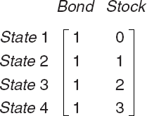
Figure 9.1. An Arrow-Debreu Market for a Stock and Risk-Free Bond; the Columns Indicate the Bond and Stock Payoffs in Different States at Time 1

In the state space model, a securities market is complete if and only if the number of linearly independent securities is equal to the number of states. The stock-bond market in Figure 9.1 is not complete because it has four states and only two securities. The bond and stock are linearly independent securities that span a two-dimensional vector space but not a four-dimensional vector space.

The state space model makes complete-markets theory operational and practical. The state space model is called the Arrow-Debreu space, and the state securities are also called the Arrow-Debreu securities and pure state-contingent claims. It is convenient to describe an Arrow-Debreu market by a payoff matrix, as the one describing a stock-bond market in Figure 9.1. The rank of the payoff matrix is a measure of market completeness. A higher rank implies greater completeness. A securities market is complete if and only if the rank equals the number of states m.

Complete financial markets benefit both the economy and society because they facilitate efficient allocation of capital and risk. Therefore, it has been a public policy in recent decades to enhance the completeness of financial markets. In particular, this public policy has fostered a rapid growth of the markets for derivative securities, especially, after Ross (1976a) demonstrated in a simple way that call and put options can be used to complete financial markets.

Let us complete the stock-bond market depicted in Figure 9.1 by introducing two call options written on the stock price S. The options have strike prices K = 1, 2, meaning that at time 1 the options pay max(0, S – K). Matrix A in Figure 9.2 shows the market payoffs in different states of the economy. The first column on the left is the risk-free bond, the second column is the stock, the third is the call option paying max(0, S −1), and the last is the call option paying max(0, S −2).

Figure 9.2. The Stock-Bond Market Is Completed by Two Stock Options

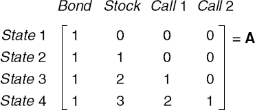
Market A is complete because is has four states and four linearly independent securities. Matrix A has an inverse A, a 4 × 4 matrix such that AA⁻¹ = I, where I is a 4 × 4 identity matrix with 1's along the diagonal and 0s off the diagonal. Therefore, the identity matrix I consists of Arrow-Debreu securities, while matrix A⁻¹ defines the composition of four stock-bond-option portfolios that replicate the Arrow-Debreu securities.

Financial derivatives have grown explosively since their emergence in the 1970s. At present, derivatives contracts are used to reallocate not only traditional risks inherent in equities, fixed income and foreign exchange, but also nontraditional risks such as corporate credit, Fed policy, housing values, commodity prices, weather conditions, political elections and others. The ability to manage and distribute risk by means of financial derivatives is partially responsible for the flexibility and resiliency that the U.S. economy demonstrates in adverse circumstances.

Market completeness simplifies valuation of financial securities. Consider a one-period Arrow-Debreu market described by an m × n matrix B, where m is the number of states and n is the number of securities. There is a risk-free bond in the market whose price P at time 0 is known. Let p be a 1 × n vector of securities prices at time 0. Then, by the no-arbitrage principle (Ross, 1976b), there exists a positive 1 ×m vector f that (in both complete and incomplete markets) justifies the following linear pricing rule:

First, the linear pricing rule implies that securities values are additive, that is, if security a is a linear combination of securities x, y, z, then the price of a is the same linear combination of the prices of x, y, z. Therefore, in a complete market, the Arrow-Debreu securities span both the time-0 price and time-1 payoffs of every security. The prices of Arrow-Debreu securities are called the state prices or Arrow-Debreu prices.

Second, in complete markets, P-f is a row-vector of Arrow-Debreu prices. The Arrow-Debreu prices can be inferred from market prices p by inverting matrix B (that has rank m in a complete market). If any state price is not positive, then there is an arbitrage opportunity in the market. Third, by linear pricing, the bond price P satisfies P = P.f.1, where 1 is a column-vector of 1s; therefore, 1 = f.1. Since f is strictly positive in the absence of arbitrage, it follows that f is a probability function defined on the state space of the market, Ω.

The linear pricing rule looks like the risk-free discounting of expected future values, which is consistent only with risk-neutral preferences. Therefore, f is called a risk-neutral probability function, risk-neutral probability measure and martingale measure. Much of modern valuation theory is devoted to the construction of risk-neutral probabilities and Arrow-Debreu prices.

In a complete securities market, a unique risk-neutral probability function obtains by inverting matrix B. In fact, market completeness can be characterized by uniqueness of risk-neutral probabilities. By contrast, incomplete markets feature multiple risk-neutral probability functions, leading to ambiguous securities prices. A way to resolve the ambiguity is to introduce utility functions that represent agents' preferences. A major advantage of arbitrage-free pricing in complete markets is that it is independent of agents' preferences.

Most single-period results generalize to multiperiod markets. A multiperiod market is a sequence of single-period markets. The states of the world in a multiperiod market are identified with different price trajectories. A multiperiod market is said to be complete if every state of the world is insurable. A multiperiod market is complete if and only if every intermediate single-period market is complete. See Pliska (1997, section 4.4) for proof and discussion.

The number of states can be very large in discrete-time markets and infinitely large in continuous-time markets. Fortunately, it takes fewer securities than the number of states to complete a multi-period market. Dynamic spanning makes it possible. Consider a multiperiod market for a stock whose price trajectories form a binary tree depicted in Figure 9.3. Every period, the stock price jumps to one of two possible states—up or down. Also, there is a risk-free bond that returns 1 in each state at the end of each period.

Since a single-period market has two states—up and down—and two linearly independent securities—stock and bond, this market is complete and every additional security is redundant; that is, it can be spanned by the stock-bond portfolio and priced by a linear combination of the stock and bond prices. Therefore, it is possible to dynamically complete the multiperiod market by rebalancing the stock-bond portfolio every single period.

The binary tree in Figure 9.3 represents eight trajectories of the stock price over three time periods and eight final states of the stock price at time 4. These states can be dynamically insured using only a stock and bond. Therefore, it takes fewer securities than the number states to dynamically complete this multiperiod market.

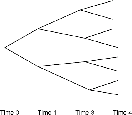
Figure 9.3. The Binary Tree Represents Potential Trajectories of the Stock Price that at Every Node Moves Either Up or Down

Dynamic rebalancing of the stock-bond portfolio is the essence of the binomial stock option pricing in Cox, Ross, and Rubinstein (1979). Since every period the stock-bond model is complete, a stock option is a redundant security that can be replicated and priced by the stock and bond. Dynamic replication of put options on stock market indices (using cash and stock-index futures) has been commercialized under the name of portfolio insurance. Portfolio insurance failed to fulfill its promise as the stock market crushed in October 1987, revealing that some risks were not insured.

A discrete-time model converges to a continuous-time model as the duration of each single period contracts to zero. In continuous time, a stock and bond are linearly independent every instant while a stock option is redundant. Since the stock, bond, and stock option are linearly dependent, each one of them can be replicated by the other two. For example, the risk-free bond can be replicated by continuous rebalancing of a portfolio that includes the stock and stock option.

This procedure is employed in the Black-Scholes stock option model. Every instant, the stock and stock option are combined in a risk-free portfolio, called the riskless hedge, that eliminates the equity risk. In the absence of arbitrage, the riskless hedge must generate the same rate of return as the risk-free bond. This no-arbitrage condition leads to an equation that is solved for the stock option price in terms of the current stock and bond prices. See Merton (1973) and Black and Scholes (1973).

Arbitrage-free valuation in complete markets is used for pricing both derivative securities and primary securities (such as stocks, bonds, and other securities in positive net supply; by contrast, exchange-traded derivatives are in zero net supply). In particular, the Black-Scholes-Merton options valuation technology has been used extensively for pricing fixed-income securities. Some examples are Vasicek (1977); Brennan and Schwartz (1979); Cox, Inger-soll, and Ross (1985); Ho and Lee (1985); Hull and White (1990); Black, Derman, and Toy (1990); and Heath, Jarrow, and Morton (1992).

Complete markets make arbitrage-free preference-free valuation feasible. The absence of market arbitrage guarantees the existence of risk-neutral probabilities that reduce asset pricing to the risk-free discounting of expected future values. See Cox and Ross (1976) and Harrison and Kreps (1979). However, the absence of arbitrage does not guarantee the existence of unique risk-neutral probabilities. In fact, in incomplete markets, there are many feasible risk-neutral measures, leading to ambiguous pricing. No-arbitrage offers unambiguous preference-free asset pricing only in complete markets.

Financial decision making in complete markets is analogous to solving a system of linear simultaneous equations when the number of unknowns equals the number of (linearly independent) equations. Such systems have unique unambiguous solutions. Whenever the number of unknowns exceeds the number of equations, there are multiple solutions, creating ambiguity and uncertainty. This situation describes incomplete markets and often prevails in the real markets.

Consider, for example, the irrelevance theorems set forth by Modigliani and Miller (1958, 1961): The firm's value is independent of the capital structure policy and dividend policy (in the absence of taxes and bankruptcy costs). In other words, changing leverage and redistributing assets should not affect the firm's value. The proof relies on the absence of arbitrage and linear pricing. As such, this proof can work only in complete markets. In reality, the Modigliani-Miller theorems often fail, and incomplete markets may be one of the reasons.

It has been known at least since Hayek (1937, 1945) that competitive market prices contain consensus expectations and other information of interest to both investors and economists. This information, however, remained inaccessible until Breeden and Litzenberger (1978) and Banz and Miller (1978) showed that risk-neutral probabilities could be inferred from options prices in complete markets. This was a pivotal discovery because it offered a practical way of decoding market prices and because risk-neutral probabilities approximate consensus probability beliefs.

The risk-neutral probability distributions implied in stock option prices have been extensively studied by Rubinstein (1994), Rubinstein and Jeckwerth (1996), Ait-Sahalia and Lo (1998), Buchen and Kelley (1996), and others. The implied risk-neutral distributions vary over time but their general properties remain the same and include a bell shape, realistic dispersions, and fat left-hand tails. Also, implied risk-neutral probabilities resemble plausible consensus beliefs. Risk-neutral probabilities recovered from the prices of fixed-income and foreign-exchange securities have similar properties.

From a technical viewpoint, extracting investor expectations from market prices is similar to identifying weather patterns, mapping out oil reservoirs, decoding noisy radio signals and other problems where a full image is to be constructed on the basis of partial observation. More complete observations generate more accurate images. In particular, greater market completeness means a more complete price set that allows for more accurate inference. In this sense, complete market prices are more informative than incomplete market prices.

Since derivative securities improve completeness, their prices represent a fertile source of recoverable market information. For example, stock index options are used to infer expected stock market volatility. Fed funds futures and options are used to infer the consensus probabilities of the future Federal Reserve policy on interest rates. Credit derivatives are used to infer the expected probabilities of bond defaults.

Let's take a sample of Eurodollar futures options and invert their market prices. The expiration price of a Eurodollar futures contract is F = 100 – y, where y is the spot rate on a three-month Eurodollar deposit at the time the futures expires. For example, if the spot is y = 5.5%, then F = 94.5. There is a liquid market for options on Eurodollar futures. Both the options and underlying futures expire at the same time. At expiration, a call option is worth max(0, F – K), where K is the contractual strike price. The strike prices are set 25 basis points apart, for example, 95.00, 95.25, 95.50, and so on.

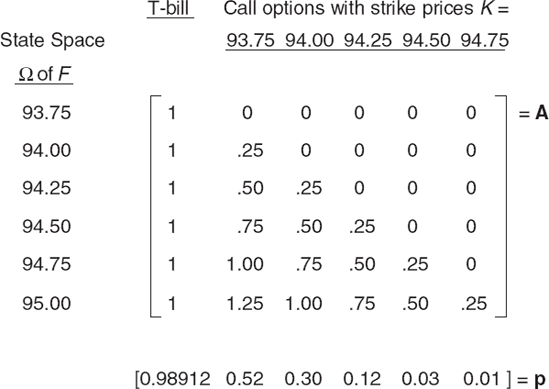
Consider a sample of Eurodollar futures options on a time interval [0, 1]. Time 0 is July 1, 1996 and time 1 is the option expiration date September 16, 1996. A set of call prices at time 0 is listed in Table 9.1, and the price of a Treasury bill, that pays $1 at maturity at time 1, is P = $0.98912.

Figure 9.4 describes an Arrow-Debreu market for five call options and the Treasury bill. The state space ω has six states indexed by possible realizations of the futures price F at time 1. The row-vector p consists of securities prices at time 0. Matrix A is the payoff matrix. The first column of A is the Treasury bill while the other columns are call options that pay max(0, F – K) at expiration. For example, zeros in the first row mean that all calls expire out of the money in the state F = 93.75. This market is complete because it has six states and six linearly independent securities.

The implied risk-neutral distribution f, obtained by inverting the payoff matrix A, is plotted in Figure 9.5. Distribution f features common properties despite a small market size. First, f is strictly positive implying no arbitrage opportunity. Second, f has a bell shape. Third, the standard deviation of the random futures price under f—about 30 bps—is a reasonable volatility estimate for short-term interest rates over two-and-half months from July 1, 1996, to September 16, 1996. Finally, f resembles plausible consensus beliefs (if it is drawn as a smooth curve).

Figure 9.4. An Arrow-Debreu Market for Eurodollar Futures Options

Figure 9.5. Risk-Neutral Probabilities f Implied in the Prices of Eurodollar Futures Options f = p.A⁻¹/P = [0.1103 0.1617 0.3640 0.2831 0.0404 0.0404]

Some additional observations are in order. First, persistent empirical properties of the implied probability distributions justify the common use of bell-shaped investor beliefs that are either postulated outright (as the normal distributions in the capital asset pricing model) or parameterized by stochastic price processes (as in many options-pricing models).

Second, while the arbitrage theory treats risk-neutral probabilities as abstract martingale measures, the empirical evidence demonstrates that the implied probability distributions resemble plausible market expectations, shaped as bell curves with realistic volatilities. Therefore, the risk-neutral probabilities are subject to some unknown conditions, yet to be discovered.

Third, it is not necessary to rely exclusively on the prices of options in order to recover the risk-neutral probabilities. For example, in Figure 9.4, the underlying futures contract can replace a call option in the payoff matrix A. Breeden and Litzenberger (1978) find an ingenious method to recover risk-neutral probabilities exclusively from options prices. In the continuous state space, the second derivative of the option premium with respect to the strike price K is proportional to the risk-neutral probability density. This follows from the continuous-space version of the linear pricing rule.

A complete market structure helps us to infer investor expectations from the prices but does not necessarily help investors to form their expectations. In other words, it is possible that the same probability beliefs prevail whether or not the market is complete. But then the same asset prices and the same portfolio allocations may exit irrespective of market completeness. An incomplete market is said to be effectively complete if it features the same prices and the same Pareto optimal allocations as a complete market. For example, removing one option from the market in Figure 9.4 leaves the market incomplete but does not necessarily cause any price changes. See Ingersoll (1987) for a discussion of effective completeness.

Uninsured states create gaps in the Arrow-Debreu space that represent missing markets as well as potential opportunities for financial innovation aimed at filling in the gaps. The notion of market completeness offers a systematic way to search for missing markets and new business ventures—find uninsured Arrow-Debreu states and create protection against the state-specific risks. Indeed, the design of housing futures, weather derivatives and other securities has followed this formula. Whether or not financial entrepreneurs are aware of the Arrow-Debreu space, their inventions tend to enhance market completeness.

Some of the new financial instruments include inflation-protected securities, mortgage-related securities, asset-backed securities, securitized insurance products, emerging markets, exchange-traded funds as well as a myriad of derivative products. Among recent investment strategies are portfolio indexing, fundamental indexing, fund-of-funds, long/short equities, market-neutral equities, event-driven trading, and other hedge-fund strategies. Electronic trading, decimalization, privatization and globalization of securities exchanges are some of the factors improving trading mechanisms and making execution faster and cheaper.

Since the early 1980s, U.S. investment portfolios have enjoyed improved allocational efficiency and solid returns thanks, in part, to diverse investment choices and risk-management tools that span the domestic Arrow-Debreu space more fully than ever. As the investment universe has extended globally, the Arrow-Debreu space has also expanded to include unfamiliar states of the world. The global state space presents new economic opportunities and risks; for example, in the fledgling markets in Southeast Asia and Eastern Europe, in the countries that ran centrally planned economies as recently as the end of the last century.

As the investment universe expands, the insights of Ross (1976a) remain as useful as ever. First, as we have discussed, Ross (1976a) proves that the (one-period) market for every primary security can be completed by calls and puts written on this security. Hence, there is no need for more complicated options than plain vanilla calls and puts. This is not, however, a cost-efficient way to hedge diversified investment portfolios because of high transaction costs and because an option on a portfolio is cheaper than a set of options on individual securities. It is more cost-efficient to use portfolio options than single-security options.

Second, Ross (1976a) proves a surprising result: given a universe of primary securities, there is a special portfolio, a Ross portfolio, such that calls and puts on this portfolio span the same space as all other options on all other portfolios. Hence, plain vanilla calls and puts on a Ross portfolio are at least as powerful as any set of simple or complex options. The linchpin is a Ross portfolio. Despite its appeal, it is unknown how to design this portfolio in practice and whether or not it is unique. As the investment universe changes, so does the Ross portfolio (or portfolios). In reality, therefore, market completeness is always a moving and elusive target.

When Ross (1976a) was published, no portfolio-based products existed; only single-stock options traded in the market. Since then, structured portfolio investments, for example, index funds and exchange-traded funds (ETFs), have gained broad acceptance, while stock index options have grown to dominate single-stock options. Moreover, certain portfolios have become busy hubs of trading activity and liquidity. For example, the S&P 500 stock index is a good proxy for a Ross portfolio. Index derivatives are used extensively even when the equity investments are significantly different from the S&P 500 portfolio.

Similarly, mortgage investors favor the liquidity of Treasury futures to hedge mortgage prepayments despite substantial basis risk (a mismatch between a hedge and the hedged), whereas several mortgage-specific contracts have failed. When investors face a choice between basis risk and liquidity risk, they usually take basis risk in order to avoid unpredictable costs of illiquidity. It is possible to create precise hedges but they will be illiquid and costly. The basis risk is clear evidence of incompleteness. Since poor liquidity causes basis risk, it also inhibits completeness. Conversely, good liquidity helps to reduce basis risk and to complete the market.

In practice, there are popular market benchmarks, for example, the S&P 500 stock index and the 10-year Treasury note, surrounded by large liquidity pools. These benchmarks occupy strategic locations in the market and in the Arrow-Debreu space—they are low-correlated (or near orthogonal) among themselves and high-correlated (or near parallel) to many other investments. As such, they deliver effective spanning and make basis risk manageable in addition to generating pools of liquidity.

The complete market theory and mean-variance theory are two main models of financial markets. In the mean-variance theory, securities are described by the means, variances, and correlations of their returns. This description is so compact that the entire securities market fits in the risk-return plane. The complete market model, by contrast, occupies a multidimensional vector space because of its detailed security format. Every mean-variance security can be reformatted and the risk-return plane can be in embedded in the Arrow-Debreu space, preserving the mathematical mean-variance properties. An economic integration of the two models is more problematic than mathematical integration.

The mean-variance theory has three parts. The first is the Markowitz (1952) portfolio model that selects investments by maximizing the expected portfolio return for a given level of volatility. The solutions, called the mean-variance efficient portfolios, form the efficient frontier depicted in Figure 9.6. The Markowitz portfolio model works in a complete market without restrictions. Moreover, mean-variance efficient portfolios correspond to Pareto optimality—new attractive securities improve al-locational efficiency and lift the efficient frontier, as shown by the dotted line in Figure 9.6.

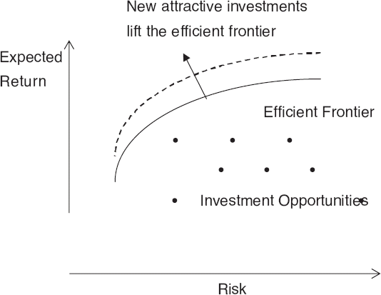
Figure 9.6. Investment Opportunities and the Mean-Variance Efficient Frontier in the Risk-Return Plane; New Attractive Opportunities Lift the Efficient Frontier

The second part is the two-fund separation: All endowments should be invested in the risk-free asset and market portfolio. The relative allocation between the two may depend on individual risk preferences but there is no need to consider any other investments. Dibvig and Ingersoll (1982) prove that in a mean-variance complete market, the two-fund separation holds only if all investors have quadratic utilities. Quadratic-utility investors can prefer less to more and can create arbitrage opportunities as a result. But arbitrage opportunities preclude market equilibrium that is germane to the mean-variance analysis. Therefore, complete markets generally do not support the two-fund separation.

The third part is the mean-variance pricing based on the capital asset pricing model. Dibvig and Ingersoll (1982) prove that, in complete markets, the mean-variance pricing is valid for primary securities but not for derivative securities. Therefore, mean-variance prices create arbitrage opportunities in a complete market that includes both primary and derivative securities. To sum up, except for the Markowitz portfolio model, the mean-variance theory is not consistent with complete markets. This conclusion may be unsettling to academics but not to professional investors, because, out of the entire mean-variance arsenal, only the Markowitz portfolio model is used extensively in practice.

Market completeness is a theoretical concept of practical importance. First, complete markets help consumers, producers and investors make efficient allocations of capital and other scarce resources; efficiently manage financial risks; and extract useful information from market prices. Second, complete markets in the Arrow-Debreu space provide the modern framework for analysis of securities markets and corporate finance. For example, arbitrage-free preference-free pricing is valid only in complete markets. Third, the complete market theory lays a road map to financial innovation, including new securities, investment strategies, and capital market architecture. In sum, few economic theories combine abstract models and practical applications as well as the complete market theory.

Ait-Sahalia, Y., and Lo, A. (1998). Nonparametric estimation of state-price densities implicit in financial asset prices. Journal of Finance 53, 2: 499–547.

Arrow, K. J. (1951). An extension of the basic theorems in classical welfare economics. In J. Neyman (ed.), Proceedings of the Second Berkeley Symposium on Mathematival Statistics and Probability (pp. 507–532), California: University of California Press.

Arrow, K. J. (1964). The role of securities in the optimal allocation of risk-bearing. Review of Economic Studies 31, 2: 91–96. (First appeared in French in 1953.)

Arrow, K. J., and Debreu, G. (1954). Existence of an equilibrium for a competitive economy. Econometrica 22: 265–290.

Black, F., and Scholes, M. (1973). The pricing of options and corporate liabilities. Journal of Political Economy 81, 3: 637–654.

Black, F., Derman, E., and Toy, W. (1990). A one factor model of interest rates and its application to Treasury bond options. Financial Analysts Journal 46, 1: 33–39.

Breeden, D., and Litzenberger, R. (1978). Prices of state contingent claims implicit in options prices. Journal of Business 51, 4: 621–651.

Brennan, M. J., and Schwartz, E. S. (1979). A continuous time approach to the pricing of bonds. Journal of Banking and Finance 3: 133–155.

Buchen, P. W., and Kelley, M. (1996). The maximum entropy distribution of an asset inferred from option prices. Journal of Financial and Quantitative Analysis 31: 143–159.

Cox, J. C., Ingersoll, J. E. Jr., and Ross. S. A. (1985). A theory of the term structure of interest rates. Econometrica 53: 385–407.

Cox, J. C., and Ross, S. A. (1976). The valuation of options for alternative stochastic processes. Journal of Financial Economics 3: 145–166.

Cox, J. C., Ross, S. A., and Rubinstein, M. (1979). Option pricing: A simplified approach. Journal of Financial Economics 7: 145–166.

Debreu, G. (1951). The coefficient of resource utilization. Econometrica 19: 273–292.

Debreu, G. (1959). Theory of Value. New York: John Wiley & Sons.

Dibvig, P. H., and Ingersoll, J. E. Jr. (1982). Mean-variance theory in complete markets. Journal of Business 55, 2: 233–251.

Harrison, J. M., and Kreps, D. (1979). Martingales and arbitrage in multiperiod capital markets. Journal of Economic Theory 20: 215–260.

Hayek, F. A. (1937). Economics and knowledge. Economica, New Series, 4, 3: 33–54.

Hayek, F. A. (1945). The use of knowledge in society. American Economic Review 35, 4: 519–530.

Heath, D., Jarrow, R., and Morton, A. (1992). Bond pricing and the term structure of interest rates: a new methodology for contingent claims valuation. Econometrica 60, 1: 77–105.

Ho, T. S., and Lee, S. (1985). Interest movements and pricing interest rate contingent claims. Journal of Finance 41, 5: 1011–1028.

Hull, J., and White, A. (1990). Pricing interest rate derivative securities. Review of Financial Studies 3, 4: 573– 592.

Ingersoll, J. E. (1987). Theory of Financial Decision Making. Savage, MD: Rowman & Littlewood Publishers.

Jackwerth, J. C., and Rubinstein, M. (1996). Recovering probability distributions from options prices. Journal of Finance 51, 5: 1611–1631.

Markowitz, H. M. (1952). Portfolio selection. Journal of Finance 7, 1: 77–91.

Merton, R. C. (1973). Theory of rational option pricing. Bell Journal of Economics and Management Science 4: 141–183.

Miller, M., and Modigliani, F. (1961). Dividend policy, growth and the valuation of shares. Journal of Business 34: 411–433.

Modigliani, F., and Miller, M. (1958). The cost of capital, corporation finance and the theory of investment. American Economic Review 48, 3: 261–297.

Pliska, S. R. (1997). Introduction to Mathematical Finance. Malden, MA: Blackwell Publishers.

Ross, S. A. (1976a). Options and efficiency. Quarterly Journal of Economics 90, 1: 75–89.

Ross, S. A. (1976b). Return, risk and arbitrage. In I. Friend and J. Bicksler (eds.), Risk and Return in Finance (pp. 189–218), Cambridge, MA: Ballinger.

Rubinstein, M. (1994). Implied binomial trees. Journal of Finance 49, 3: 771–818.

Vasicek, O. (1977). An equilibrium characterization of the term structure. Journal of Financial Economics 5: 177– 188.