
JEFFREY D. FISHER, PhD
Dunn Professor of Real Estate, Indiana University
DAVID GELTNER, PhD
George Macomber Professor of Real Estate Finance, MIT
Abstract: Despite the tremendous growth in the use of derivatives for commodities, stocks, interest rates, currency and other applications, the availability of derivatives for commercial real estate has been limited. When you consider that real estate assets comprise over one-third of the value of all of the underlying physical capital in the United States and the world, the potential for real estate derivatives is impressive. It is therefore not surprising that in recent years real estate derivatives have begun to develop, as market participants have realized the role that derivatives can play, investment banks have been willing to offer derivatives, and new indices have been developed that are designed to meet the needs of the evolving real estate derivatives market.
Keywords: derivatives, forward, swaps, indices, hedge, alpha, short, structured notes, counterparty
This chapter discusses the type of derivatives now being offered for commercial real estate including total return swaps, forward contracts, and structured notes. Such products address several of the classical problems that have been raised regarding real estate investment, including: high transactions and management costs, lack of liquidity, inability to sell short, and difficulty making well-diversified property investments whose returns are measured in a manner comparable to those of stocks and bonds. This chapter also discusses the fundamentals of real estate return indices used to support derivatives including the both appraisal-based and transactions-based indices. A discussion of pricing of commercial real estate derivatives is provided in Chapter 52 of Volume III.
There are a myriad of potential uses of real estate derivatives by different market participants. Examples are exposure to the real estate asset class, hedge existing exposure, harvesting alpha, portfolio balancing, real value investing, and efficient leverage.
Derivatives provide a way for investors to get exposure to the commercial real estate asset class relatively quickly, with relatively low transaction or management costs and relatively high diversification. This can be particularly useful for investors who lack the expertise to either purchase and manage individual properties directly, or find and manage specialized investment managers or real estate property funds. For example, a foreign investor who wants immediate, well-diversified exposure to the U.S. real estate market may want to take a long position on a real estate derivative such as a forward contract or a swap that is based on a national real estate index. Purchasing the derivative results in the equivalent of exposure to a well-diversified portfolio of properties and hence very little if any unsystematic risk without incurring the costs of purchasing and managing properties. Similarly, a small pension fund may want exposure to a well-diversified portfolio of real estate but lacks the scale to purchase enough individual properties to be well diversified by property type and location, and lacks the expertise to choose among property funds with their various investment management and transaction fees.
Investment managers who find they are over exposed to the real estate asset class, perhaps because real estate has performed well compared to their stock and bond portfolio, or because they have a relatively bearish outlook for real estate, may want to take a short position in a derivative to reduce their exposure to real estate without the need to sell properties, or until transactions can be completed on the sale of properties (which can take time to market and close). Shorting the derivative can also lock in profits made in the real estate market so the investment manager doesn't risk a drop in value before the properties can be sold. Lenders and originators of commercial mortgage-backed securities, exposed to either "warehouse" or portfolio risk, can hedge using a short positions in forwards or swaps, or by purchasing a put option, based on real estate indices. Credit default swaps can also be designed that result in a payoff to the party purchasing the swap that is triggered by the index's declining below a certain level.
Real estate investment managers who have the expertise to acquire, manage, and sell properties so as to persistently outperform the real estate market can monetize such positive alpha without selling properties, and produce profitable returns even when the real estate market turns down, by using the short position in the derivative to effectively "cover" their real estate market exposure, a "risk management" tool that acts effectively like real estate market value "insurance." This allows the investment manager to focus on their area of specialized expertise and comparative advantage, dealing and managing in the real estate market, regardless of the current ebbs or flows in the capital markets.
Real estate portfolio managers may also feel that their allocation to different property types or geographic locations has gotten out of balance. For example, they may feel that they are overexposed to office properties and under exposed to retail properties. They may enter into a swap with a counterparty where they pay the office returns on an index of office properties and receive the return on an index of retail properties. Similarly, an investor could swap returns on an index of properties in the east with an index of properties in the west.
Hedge funds and other more opportunistic investors may feel that they can identify which property sectors or geographic locations will outperform others. Thus, they may enter into different long and short positions on derivatives to try to capture the perceived mispricing. They would not necessarily have any desire to own and manage the physical real estate.
As forward and futures contracts do not in themselves require up-front cash investment, such derivatives can be used in effect to take levered positions in real estate if the investor does not fully cover the derivative position with bond investment. Depending on circumstances, this may present a lower-cost method of levering the investment, compared to traditional real estate debt.
A foreign investor wants to quickly get exposure to the U.S. real estate market to diversify into the United States but does not have the time and expertise to identify individual properties and be sure he is also diversified within the United States. He enters into a long position on a two-year forward contract based on a national real estate index. The index is currently at 100. He has seen forecasts for the index ranging from 105 to 115 in two years. He agrees on a forward price of 105 that he will pay at the end of the two years in order to receive a payment based on the actual change in the index. The contract pays $500,000 times the index value. No cash payment is made today, although a margin or bond may be required. The magnitude of the required margin or bond posting is relatively small and may earn interest. The required posting would normally be related to the likely magnitude of change in the value of the index over the relevant derivative contract period, rather than to the magnitude of the overall notional amount of the trade, and thus allows the investor to obtain very high effective leverage unless the notional amount of the trade is otherwise covered by up-front cash investment (e.g., in bonds).
Suppose that at the end of the two years the index is 115 (upper end of forecast). The investor will receive $500,000 × (115 − 105) = $5 million. However, if at the end of the two years the index is 95 (bad forecast!) the investor will pay $500,000 × (95 − 105) = -$5 million.
There will also be a counterparty to the above transaction who has the short position—the other side of the position the foreign investor took. The short position receives the opposite cash flows in the previous example, receiving $5 million when the index is 95 and paying $5 million when it is 115. The short might be, for example, a commercial mortgage-backed security (CMBS) issuer who wants to hedge its warehouse risk, a hedge fund that believed the low end of the forecast was more likely, or an investment manager seeking to "harvest alpha" (explained next). The CMBS issuer trying to hedge "warehouse risk" (loan pools or securities held temporarily awaiting sale) would probably prefer to use a periodically cash-settled swap rather than a two-year forward (because "warehoused" loans are not held very long, though the CMBS issuer may typically always have some warehoused loans on hand). Swaps will be described shortly.
A specialized real estate asset management fund believes it can purchase, manage, and sell properties so as to consistently outperform the real estate index that underlies the derivative (and with same risk), based on the manager's specialized expertise. They want to harvest this positive "alpha" from these excess returns whether the market is up or down. Since the investment manager cannot control the market, but can (presumably) control its alpha (based on its specialized expertise), the idea is for the manager to profit from the activity they can control and are particularly good at, while laying off risk exposure to factors they cannot control. This is a classical type of "risk management" for an investment management firm. To hedge exposure on $50 million worth of properties the manager owns, for example, the manager would sell (short) $50 million notional value of the forward contract on the index that we described in the previous example. For that portion of the fund's property holdings, the fund is "market neutral": they have laid off their "beta" market risk exposure by their offsetting positions in the forward short and their covering property holdings. This leaves them with only their alpha, the difference between their property performance and the market (index) performance, and with any "basis risk," systematic or nonsystematic differences between the ex post performance of their property holdings and the market (index) not due to the manager's actions.
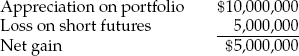
Suppose at the end of the two years the fund's portfolio increased in value by 20% (including income reinvested in the fund). Suppose the index rose to 115 over the two years (that is, the fund beat the index by 500 basis points).
Suppose at the end of the two years the hedge fund's portfolio decreased in value by 2%, while the index decreased to 95 (that is, the fund beat the market by 300 basis points).
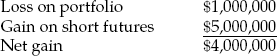
The fund thus gains in this example between $4 and $5 million whether the market increases or decreases, based purely on the positive alpha obtained on the fund's properties. In this extreme example of fully hedging the $50 million amount (and with no basis risk), the fund has been turned into an "alpha machine" that makes (or loses) money purely on its differential performance relative to the index, a differential that purely reflects the fund manager 's particular expertise and skill at the property and deal level relative to the index. This "disarticulates" performance based on real estate expertise from performance based on the movements and forces and flows of the broader financial capital market that may move the real estate asset market one way or another at any given time.
An open-ended fund has funds to invest but has not identified properties they wanted to purchase. They believe that the return on an index that tracks changes in property values will be stronger over the next two years than most market participants believe. They decide to take a long position in a real estate index capital return as a swap where they receive the index capital return and pay a fixed leg each quarter. Recall that the capital return is the change in property value. Suppose they can purchase the capital return and pay a fixed leg of 50 basis points. The notional amount of the swap is $100 million. Suppose the actual capital return over the next eight quarters is as shown in Table 51.1. In the first quarter the capital return is 2% so the fund receives 2% of $100 million or $2 million. They pay 0.5% of $100 million or $500,000 on the fixed leg. Thus, they net $1.5 million. Note that in the last four quarters they end up paying money because the capital return did not cover the fixed leg. They end up netting zero over the eight quarters, no doubt not as well as they had hoped in this case, but this reflects the real estate market risk that is represented in the index. Perhaps the market performed worse than this investor had hoped, or perhaps they agreed to a fixed leg that was too high.
Creating derivatives for commercial real estate requires the availability of indexes that are the basis for calculating the payoffs to the parties in the derivative transaction. The oldest index for commercial real estate investment performance in the United States is the NCREIF Property Index (NPI) published by the National Council of Real Estate Investment Fiduciaries. The NPI is an appraisal-based index that has returns available on a quarterly basis since 1978 and as of the end of 2006 included almost $250 billion in real estate. More recently other indexes have been created to meet the needs of having a viable derivative market in the United States, including indices based on real estate transactions developed initially at the Massachusetts Institute of Technology (MIT).
In order to have good derivative contracts, we need good indices underlying the contracts. A property derivative contract is no better than the index on which it is based. It is probably impossible to have a perfect index to use for commercial real estate derivatives. Unlike stock indices that can be used for futures contracts, it is not possible to invest in all or even a few of the properties used for a real estate index because the properties are held by many different investors in different types of investment vehicles that are privately held. Furthermore, properties do not transact on a frequent basis like stocks to be able to simply measure the change in value of each property in the index based on daily, monthly, quarterly, or even annual transaction prices. There are two main ways of dealing with the fact that the same property does not transact frequently. The first is to have an index based on appraisals of the property on a quarterly basis. This is the basis for the NCREIF property index mentioned above. The second way of creating an index is to base it on the transactions that do occur for properties and have the model control for the varying time between sales of properties.
Table 51.1. Actual Capital Gain Returns for Illustration
Quarter | Capital Return | Long Receives ($ million) | Long Pays ($ million) | Net to Long ($ million) |
|---|---|---|---|---|
1 | 2.00% | $2.0 | $0.5 | $1.5 |
2 | 1.50% | $1.5 | $0.5 | $1.0 |
3 | 1.00% | $1.0 | $0.5 | $0.5 |
4 | 0.50% | $0.5 | $0.5 | $0.0 |
5 | −1.00% | -$1.0 | $0.5 | -$1.5 |
6 | 0.00% | $0.0 | $0.5 | -$0.5 |
7 | 0.50% | $0.5 | $0.5 | $0.0 |
8 | −0.50% | -$0.5 | $0.5 | -$1.0 |
No single index is likely to be best for all trading purposes. The informational complementarities of different types of commercial property indexes, combined with the diversity and heterogeneity in the U.S. commercial property market and real estate industry, suggests that there can be value from having more than one type of index available. Use of derivatives in "arbitrage" trading across indices can be a source of profit, price discovery, and liquidity.
Real estate indices, especially appraisal-based indices, tend to be more predictable than stock market indices. Derivative prices can reflect forecasts for the underlying index. Commodity futures contracts have always reflected consensus forecasts of where the corresponding commodity spot markets are headed. Because there is momentum in a real estate index, the equilibrium (or "fair") pricing of its derivatives in the derivatives market must reflect the index predictability implied by such momentum. This differs from typical stock market index derivatives in which the underlying indices have relatively little momentum and the stock shares on which the indices are based are directly traded in liquid cash (or "spot") markets, allowing execution of arbitrage between the futures and spot markets.
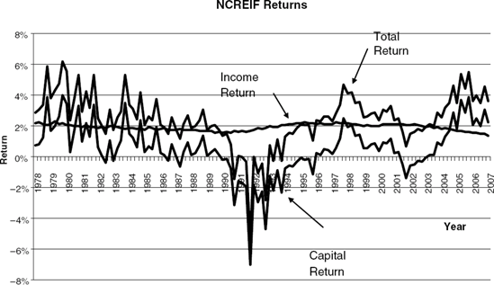
Periodic total returns for commercial real estate that reflect overall investment performance come from both the current cash flow generated by properties (income return) and changes in the capital value of the properties between the beginning and end of each index reporting period (capital return). Compared to capital returns and to most financial series, income returns are very nearly constant over typical trading periods. This is because in long-lived assets such as real property the current income per period is at least an order of magnitude smaller than the capitalized asset value. In the NPI, the quarterly volatility of the capital return between 1978 and 2006 was 1.7% versus only 0.3% for the income return. (This compares to quarterly volatility over the same historical period of 0.8% for Treasury bills, 6.8% for real estate investment trust [REIT] stocks, and 7.7% for the Standard & Poor's (S&P) 500 large-cap stock index.) Figure 51.1 shows the NPI return components (income, capital, and total) from 1978 through 2006 (quarterly unleveraged returns), revealing how the income return is essentially constant compared to the capital or total return components.
If the underlying index reports the total return (as in appraisal-based indices such as the NCREIF or Investment Property Databank [IPD] indices), then derivatives can be structured based on either the total return or just the capital return. However, even if the underlying index reports only the capital return, derivatives can effectively be used to create the total return synthetically, because virtually all of the index total return volatility is in the capital return component alone. In the NPI, over 116 quarters during 1978-2006, the capital return and total return were correlated +99%, with essentially equal volatilities of 1.7% each. For example, a structured note in which the investor funds up front the fixed leg of a capital return swap will effectively provide the investor with the index total return, as we will see later when we discuss swap pricing.
The first regularly produced commercial property price indexes were appraisal based, and designed for benchmarking institutional real estate investment manager performance. These include the NPI in the United States and the IPD Index in Great Britain, among others worldwide. In a traditional appraisal-based index all of the properties in the index population are reappraised frequently, and the index periodic returns are based on the average (usually value weighted) of those appraisal-based returns each period. This is similar to the way many institutional real estate investment funds "mark to market" their asset values and correspondingly report quarterly returns to their investors. Of course, the NPI reflects property-level returns (unlevered, and before any fund-level or management expenses and fees to which investors are subject).
While such traditional appraisal-based indices can be excellent tools for benchmarking investment manager performance, and this in itself gives them a particular use in derivatives of interest to such managers, they do have some inherent problems from the perspective of a broader derivative support role. The appraisal process tends to be somewhat subjective and backward looking (perhaps more so in the United than in Britain). This tends to impart a lag bias to the property values and the index returns. Furthermore, in the case of the NCREIF Index in the United States, not all properties are reappraised every period that the index is reported, and this adds an additional "stale appraisal" effect into the index. In the NCREIF Index, at least during some periods of its history, greater frequency of reappraisals in the fourth calendar quarter has imparted an artificial seasonality to the index (the index can tend to "spike" in the fourth quarter). It must also be recognized that, at least as of the early 2000s, the NCREIF Index represents a relatively narrow segment of the population of U.S. properties. In 2006 the NCREIF population of properties consisted of less than 10% of the commercial properties in the United States, a much smaller percentage than the IPD Index represents in Britain. For example, in 2006 the NPI included less than $30 billion of property sales, whereas the Real Capital Analytics Inc. (RCA) database recorded over $330 billion of commercial property sales tracking only sales of greater than $2.5 million. As of the end of 2006, the NPI was tracking some $250 billion worth of property, whereas J. P. Morgan Asset Management's "Real Estate Universe" report estimated the total value of U.S. commercial real estate at that time to be some $6.7 trillion, or over 25 times the NCREIF population value (although this included corporate real estate and small "mom-and-pop" properties as well as the larger properties covered by the RCA database). For smaller market segments, there may be only a few NCREIF properties available in the index, and their specific identities will be known to at least some potential participants in the derivatives marketplace.
The above problems are of less concern for purposes of benchmarking institutional real estate portfolios that are marked to market using appraised values, but they can be more problematic for broader derivative support purposes. If the lag in the index causes it to still rise when the real estate market turns down (or vice versa), this can be confusing to parties trying to use the index to hedge or speculate on such market movements. Derivative pricing when the index is lagged needs to reflect the lag, and that may make price discovery more difficult, potentially hampering liquidity in the derivative market, although in principle the lag can be relatively easily reflected in the derivative price (especially if indices that are not lagged are also available as information sources). Even if the index lag is taken into account in the derivative price, if the derivative contract expires before the lagged price movement is fully reflected in the index, then the hedge will not be complete, presenting a type of "basis risk" for the user of the derivative. Thus, for a variety of reasons, futures traders may prefer indexes that lead the appraisal-based indices in time, and in which the true volatility is not dampened, as such volatility can be a source of potential profit that might motivate some derivative traders.
An alternative to appraisal-based indices is to have an index based on transactions (sales) of properties. In principle, such indices can be based on the entire population of commercial properties, because all properties potentially transact (providing a random price sample of the population each period), whereas only certain specialized portfolios of properties are regularly marked to market in the U.S. using appraisals. Transactions-based indices can be good bases for derivatives provided the indexes are carefully constructed based on sufficient quantity and quality of transactions observations data and state-of-the-art statistical procedures to control for "apples versus oranges" differences in properties trading in different periods and to minimize "noise" or random deviations from the property population prices.
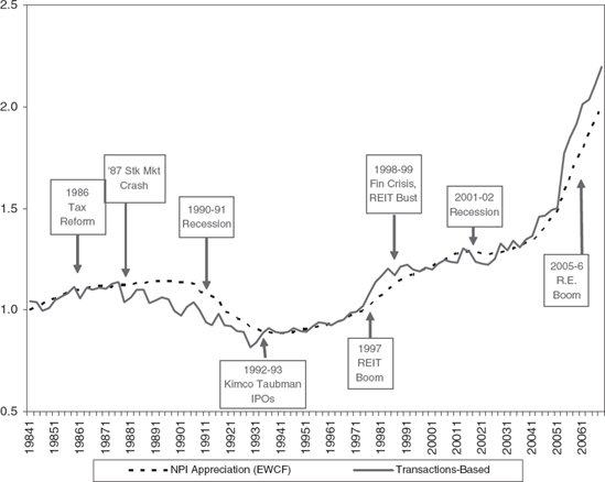
Figure 51.2. Appraisal-Based vs. Transaction-Based Capital Value Index Based on NCREIF: 1984-2006 Source: Fisher, Geltner, and Pollakowski (2007).
There are two major procedures to calculate transactions-based indices in a statistically rigorous manner: (1) the repeat-sales regression procedure and (2) the hedonic value model. Both procedures address the fundamental problem in the construction of a transactions based real estate price index, the fact that the properties that transact in one period are generally not the same as the properties that transacted in the previous period, making a direct comparison of prices "apples versus oranges." The two procedures address this issue in different ways.
The hedonic procedure models property prices as a function of various characteristics of the properties that affect their value, such as age, size, location, building quality, and so on. By regressing property transaction prices onto these "hedonic characteristics" of the properties that sell, and controlling for or keeping track of the time of the sale, one constructs a "constant-quality" price-change index or an index that tracks property market price changes controlling for differences in the properties that transact at the different points in time. The MIT Center for Real Estate began publishing the first regularly produced hedonic index of commercial property in 2006, in cooperation with NCREIF, based on the prices of the properties sold from the NCREIF Index. This transactions-based index uses the recent appraised values of the sold properties as a "composite" indicator of the hedonic characteristics of the properties, controlling in this way for cross-sectional differences in the sold properties. Because this transactions based index was based on the same underlying population of properties as the NPI, it can present a good "apples-to-apples" comparison of the difference between a transactions-based and an appraisal-based index. This comparison over the historical period from 1984 to 2006 is shown in Figure 51.2. The comparison gives an indication of the typical differences between a transactions based and an appraisal based index. Note that the transactions based version of the NCREIF Index is a bit more volatile, and tends to slightly lead the NPI in time (in terms of the timing of major turning points in the index history).
Repeat-sales indices use a different approach to address the "apples-versus-oranges" problem. As the name suggests, repeat-sales indices rely on individual properties selling more than once, so that the change in price between sales provides an indication of how same-property values have changed over time. The index is thus based on the type of price changes that investors in properties actually experience, and the same type of price changes that stock market indices are based on. Stock market indices are also based on comparing the transaction prices of stock shares in one period with the transaction prices of similar shares in the previous period. As stock shares are homogeneous (a share of IBM that traded this month is the same as a share of IBM that traded last month), the result is comparable to a "same property" price change index such as the repeat-sales transactions-based indices. It should also be noted that stock share prices reflect the value added by the corporation not paying out all of its cash in dividends, but reinvesting some in the corporation. This is analogous to the effect of capital improvement expenditures in real estate. Thus, repeat-sales indices aimed at tracking property prices do not generally try to remove the effect of capital improvement expenditures (although normally data filters are applied to eliminate property sale pairs that would reflect major development, redevelopment, or rehabilitation of the properties). This is in some contrast to appraisal-based indices that may subtract capital expenditures from the appreciation return reported by the index.
The statistical process used to calculate repeat-sales indices takes into consideration the time between the same-property sales and appropriately allocates the price change to each period that the index is reported, based on information from other repeat sales occurring over various time frames. Repeat sales is the approach used in widely quoted housing price indices such as the S&P/Case-Shiller housing index on which the Chicago Mercantile Exchange (CME) launched futures trading in 2006. A simple numerical example of how the calculation process works is presented in the appendix to this chapter.
The first regularly published repeat-sales transactions based index for commercial property was developed by the MIT Center for Real Estate based on data from the firm Real Capital Analytics Inc. (RCA) and launched in 2006. This index was based on a much broader property population than the appraisal-based NCREIF Index, as the RCA database attempted to track all commercial property sales in the United States of over $2.5 million, whereas the NPI tracked only the NCREIF members' properties.
This chapter has reviewed the nature and mechanics of the major real estate equity index derivative products and their use and usefulness. It has also presented the fundamentals of real estate return indices, including the important differences between the two major types of indices: appraisal-based and transactions-based indices.
In this appendix we present a simple numerical example of the mechanics of how the repeat-sales regression procedure works to construct an index of periodic capital returns based on same-property price changes. In so doing, we will also highlight some key features of the repeat-sales model that are not intuitively obvious, such as how the model can detect a downturn in the market even when all of the individual property investments are producing a positive return over their holding periods, and how no single period's return estimate is based only on the second-sales occurring in that period alone.
To understand how the repeat-sales regression (RSR) index construction process works, you must step back briefly and recall some basic statistics. You may recall that regression analysis is a statistical technique for estimating the relationship between variables of interest. In a regression model, a particular variable of interest, referred to as the dependent variable, is related to one or more other variables referred to as explanatory variables. The regression model is presented as an equation, with the dependent variable on the left-hand side of the equal sign and a sum of terms on the right-hand side, consisting of the explanatory variables each multiplied by a parameter that is estimated by the regression and that relates each explanatory variable to the dependent variable. For example, if the dependent variable is labeled "Y" and there is a single explanatory variable labeled "X," then a simple regression model of Y as a function of × would be expressed as:
The model says that the value of the variable Y equals the value of the variable × times the parameter "a," and we would use the regression analysis of relevant empirical data to estimate what is the value of "a.". This process is referred to as "estimation" of the regression, or "calibrating" the model.
How can this technique enable the development of a real estate price index? Let's take a very simple numerical example. Suppose that the true returns in the market are respectively: 0%, +10%, and —5%, in three consecutive periods (say, 2011, 2012, and 2013). Thus, a true price index starting out at 1.00 at the end of 2010 would remain at 1.00 at the end of 2011, jump to 1.10 in 2012, and then fall back to 1.045 in 2013 [as (1.045 − 1.10)/1.10 is −5%]. Now suppose we have three property repeat-sales observations involving altogether at least one sale in each of the three years, with each being consistent with the true returns but in which no one observation can directly reveal any one period's return because the properties are held across more than one period. Property 1 is bought at the beginning of 2011 for $100,000 and sold after three years at the end of 2013 for $104,500. Property 2 is also bought at the beginning of 2011, but for $200,000 and sold at the end of 2012 for $220,000 (held for two years). Property 3 is bought at the beginning of 2012 for $300,000 and sold at the end of 2013 for $313,500 (also held two years). This is summarized in the Table 51.2 and Figure 51.3, where the figure indicates both the true market price index (the solid line) and the capital returns achieved by each of the three investors in these three properties (dashed lines).
Now let's apply the RSR model to this problem. Let the dependent variable, "Y," be the natural log of the ratio of the second sale price divided by the first sale price, for each repeat-sale pair. Thus, the first repeat-sales observation, based on Property 1, has a Y value of the log of 1.045.
Table 51.2. Prices Observed at Ends of Years
2006 | 2007 | 2008 | 2009 | |
|---|---|---|---|---|
True price index | 1.00 | 1.00 | 1.10 | 1.045 |
True capital return | 0% | 10% | −5% | |
Property 1 | $100,000 | No Data | No Data | $104,500 |
Property 2 | $200,000 | No Data | $220,000 | No Data |
Property 3 | No data | $300,000 | No data | $313,500 |
Similarly, the second repeat-sales observation, based on Property 2, has a Y value of the log of 1.10, and so on.
On the right-hand side of our RSR model, instead of just one variable, "X," let there be three variables, corresponding to the three consecutive periods of time for which we want to construct the index periodic returns. Let us label these "X2011," "X2012," and "X2013." These right-hand-side variables are what are called "dummy variables," which means they take on a value of either zero or one. The "X2011" variable stands for the year 2011. It takes the value of one if 2011 is after the year of the first sale and before or including the year of the second sale in the repeat-sales observation (in other words, if the dummy variable's year is during the property investor's holding period between when he bought and sold the property of the observation in question); otherwise, this dummy variable has a value of zero. Similarly, "X2012" takes the value of one if 2012 is after the year of the first sale and before or including the year of the second sale. Thus, the price observation data described previously gives the RSR estimation data in Table 51.3. For example, for the repeat-sales observation corresponding to Property 3, $313,500/$300,000 is 1.045, and the natural log of this value happens to be about 4.4%, which is therefore the Y value for that observation in the RSR estimation database.
Our regression equation can now be expressed as:
Now recall from statistics that the estimation of a regression model—that is, the "calibration" of the value of the parameters in the preceding equation—is mathematically the solution of a system of simultaneous equations. Each equation corresponds to one "observation," one data point in the database used to estimate the regression model. Thus, in our present example, we have three equations, one corresponding to each row (each repeat-sales observation) in Table 51.3. The three equations are:
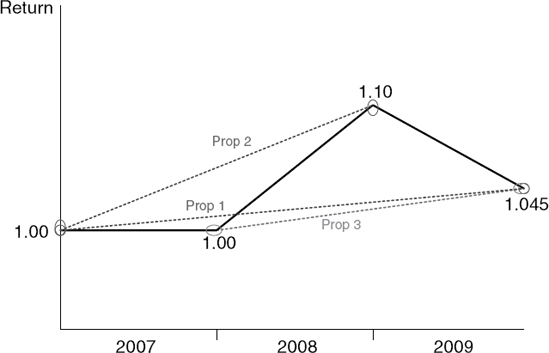
Table 51.3. RSR Estimation Data
Y Value = LN(Ps/Pf) | X2011 Value | X2012 Value | X2013 Value | |
|---|---|---|---|---|
Observation 1 | LN(1.045) | 1 | 1 | 1 |
Observation 2 | LN(1.10) | 1 | 1 | 0 |
Observation 3 | LN(1.045) | 0 | 1 | 1 |
which equates to:
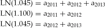
We thus have three linear equations with three unknowns (a2on, a2oi2, and a2oi3, representing the true log price ratios in each of the three periods). Such a system can always be solved, and in this case the solution can be found as follows:
| Use equation (51.2) to derive: a2012 = LN(l.l) – a2011. Then plug this into equation (51.3) to obtain: a2013 = LN(1.045) - LN(l.l) + a2011. Now plug both of these into equation (51.1) to obtain: |
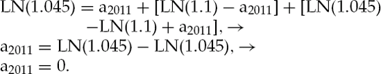
Now plug this result back into equations (51.2) and (51.3) to obtain: a2012 = LN(l.l), and a2013 = LN(1.045) – LN(l.l). The result that a2011 = 0 simply means that the estimated price index level did not change during 2011. From the definition of logarithms we have 0 = LN(1), and algebraically we can express this as LN(1/1). Similarly, we can express a2012 = LN(l.l) as LN(1.1/1). Thus, the implied log price ratios of the price index ending values divided by its beginning values each year are:
| For 2011 = a2011 =LN(1/1) |
| For 2012 = a2012 = LN(1.1/1) |
| For 2013 = a2013 = LN(1.045/1.1) |
Exponentiating these values, we arrive at the implied straight level price index as of the end of each year as follows:
| 2006 = 1.000 |
| 2007 = 1.000 |
| 2008 = 1.100 |
| 2009 = 1.045 |
with the resulting implied price-change percentages (capital returns):
| 2007 = 0% |
| 2008 = +10% |
| 2009 = −5% |
Thus, we see that the repeat-sales model has derived the true capital return in each period, even though no single repeat-sale price change observation corresponded to any one year. The model correctly derived the negative return in 2013, even though none of the repeat-sale observations used in the estimation showed a negative price change in itself. In other words, all of the three investors made a positive resale gain over their holding periods. Note also that the estimation of the returns in each of the three periods was affected by all three of the repeat-sale observations. For example, the estimate of the negative 5% return in 2013 was determined in part by the +10% return obtained on Property 2, even though that property's second sale occurred prior to the beginning of 2013.
While this is a simple numerical example, the type of result shown here is general. In principle, the repeat-sales model only requires one sales observation per period (either a first or second sale) in order to be able to estimate the true return each period, even though no single repeat-sale pair corresponds to any one period. And the model uses all observations to estimate every period's return. Thus, it is not correct to think that the estimated return in the current period is determined solely or in isolation by the second-sale observations that occur only in the current period.
Of course, in the real world, individual transaction prices will be dispersed randomly around the average (normalized) sale price at any given time, which makes index estimation a statistical process. The existence of more than one observation (hence more than one equation) in each period of time enables such estimation to be optimized in various ways, as is done in actual RSR indexes.
Bailey, M., Muth, R., and Nourse, H. (1963). A regression method for real estate price index construction. Journal of the American Statistical Association 58: 922-942.
Court, A. (1936). Hedonic price indices with automotive examples. In The Dynamics of Automobile Demand. Detroit: General Motors Corporation.
Fisher, J. D. (2005). Introducing the NPI based derivative: New strategies for commercial real estate investment and risk management. Journal of Portfolio Management, Special Issue on Real Estate: 1-9.
Fisher, J. D., Geltner, D., and Webb, R. B. (1994). Value indices of commercial real estate: A comparison of index construction methods. Journal of Real Estate Finance & Economics 9, 2: 137-164.
Fisher, J, Geltner, D., and Pollakowski, H. (2007). A quarterly transactions-based index of institutional real estate investment performance and movements in supply and demand. Journal of Real Estate Finance and Economics 34, 1: 2007.
Geltner, D., and Pollakowski, H. (2006). A set of indexes for trading commercial real estate based on the Real Capital Analytics Database. Report by the MIT Center for Real Estate.
Geltner, D., and Fisher, J. D. (2007). Pricing and index considerations in commercial real estate derivatives.
Goodman, L. S., and Fabozzi, F. J. (2005). CMBS total return swaps. Journal of Portfolio Management, Special Issue on Real Estate: 162-167.
Griliches, Z., and Adelman, I. (1961). On an index of quality change. Journal of the American Statistical Association 56: 535-548.
Rosen, S. (1974). Hedonic prices and implicit markets. Journal of Political Economy 82,1: 33-55.