
FRANK J. FABOZZI, PhD, CFA, CPA
Professor in the Practice of Finance, Yale School of Management
ANAND K. BHATTACHARYA, PhD
Managing Director, Countrywide Securities Corporation
WILLIAM S. BERLINER
Executive Vice President, Countrywide Securities Corporation
Abstract: The mortgage market in the United States has emerged as one of the world's largest asset classes. The growth of the mortgage market is attributable to a variety of factors. Most notably, strong sales and price growth in the domestic real estate markets and the increased acceptance of new loan products on the part of the consumer has dovetailed with the acceptance of a variety of loan products as collateral for se-curitizations. Due to a variety of reasons such as product innovation, technological advancement, and demographic and cultural changes, the composition of the primary mortgage market is evolving at a rapid rate—older concepts are being updated, while a host of new products is also being developed and marketed. Consequently, the mortgage-lending paradigm continues to be refined in ways that have allowed lenders to offer a large variety of products designed to appeal to consumer needs and tastes. This evolution has been facilitated by sophistication in pricing that has allowed for the quantification of the inherent risks in such loans. At the same time, structures and techniques that allow the burgeoning variety of products to be securitized have been created and marketed, helping to meet the investment needs of a variety of market segments and investor clienteles.
Keywords: mortgage, servicers, lien status, prime loans, subprime loans, alternative-A loans, credit scores, loan-to-value ratio (LTV), documentation, fixed-rate mortgages, adjustable-rate mortgages (ARMs), hybrid ARM, interest-only (IO) mortgage, government guarantees, conventional loans, guaranty fee, prepayments, refinancing, curtailment, negative convexity, delinquencies, defaults, loss severity
The purpose of this chapter is to explain mortgage products and their investment characteristics. The chapter introduces the basic tenets of the primary mortgage market and mortgage lending, and summarizes the various product offerings in the sector. This chapter provides a framework for understanding mortgage-backed securities (MBSs).
In general, a mortgage is a loan that is secured by underlying assets that can be repossessed in the event of default. For the purposes of this chapter, a mortgage is defined as a loan made to the owner of a one- to four-family residential dwelling and secured by the underlying property (both the land and the structure or "improvement"). After issuance, loans must be managed (or "serviced") by units that, for a fee, collect payments from borrowers and pass them on to investors. In addition to managing and tracking payments, servicers are also responsible for interfacing with borrowers if they become delinquent on their payments, and also manage the disposition of the loan and the underlying property if the loan goes into foreclosure.
There are a number of key attributes that define the instruments in question that can be characterized by the following dimensions:
Lien status, original loan term
Credit classification
Interest rate type
Amortization type
Credit guarantees
Loan balances
Prepayments and prepayment penalties
We discuss each below.
Lien Status
The lien status dictates the loan's seniority in the event of the forced liquidation of the property due to default by the obligor. A first lien implies that a creditor would have first call on the proceeds of the liquidation of the property if it were to be repossessed. Borrowers often utilize second lien or junior loans as a means of liquefying the value of a home for the purpose of expenditures such as medical bills or college tuition or investments such as home improvements.
Original Loan Term
The great majority of mortgages are originated with a 30-year original term. Loans with shorter stated terms are also utilized by those borrowers seeking to amortize their loans faster and build equity in their homes more quickly. The 15-year mortgage is the most common short-amortization instrument, although issuance of loans with 20- and 10-year terms has grown in recent years.
Credit Classification
The majority of loans originated are of high-credit quality, where the borrowers have strong employment and credit histories, income sufficient to pay the loans without compromising their creditworthiness, and substantial equity in the underlying property. These loans are broadly classified as prime loans, and have historically experienced low incidences of delinquency and default.
Loans of lower initial credit quality, which are more likely to experience significantly higher levels of default, are classified as subprime loans. Subprime loan underwriting often utilizes nontraditional measures to assess credit risk, as these borrowers often have lower income levels, fewer assets, and blemished credit histories. After issuance, these loans are typically serviced by special units designed to closely monitor the payments of subprime borrowers. In the event that subprime borrowers become delinquent, the servicers move immediately to either assist the borrowers in becoming current or mitigate the potential for losses resulting from loan defaults.
Between the prime and subprime sector is a somewhat nebulous category referenced as alternative-A loans or, more commonly, alt-A loans. These loans are considered to be prime loans (the "A" refers to the A grade assigned by underwriting systems), albeit with some attributes that either increase their perceived credit riskiness or cause them to be difficult to categorize and evaluate.
Mortgage credit analysis employs a number of different metrics, including the following.
Credit Scores Several firms collect data on the payment histories of individuals from lending institutions and use sophisticated models to evaluate and quantify individual creditworthiness. The process results in a credit score, which is essentially a numerical grade of the credit history of the borrower. There are three different credit-reporting firms that calculate credit scores: Experian (which uses the Fair Isaacs or FICO model), Transunion (which supports the Emperica model), and Equifax (whose model is known as Beacon). While each firm's credit scores are based on different data sets and scoring algorithms, the scores are generically referred to as FICO scores.
Loan-to-Value Ratios The loan-to-value ratio (LTV) is an indicator of borrower leverage at the point when the loan application is filed. The LTV calculation compares the face value of the desired loan to the market value of the property. By definition, the LTV of the loan in the purchase transaction is a function of both the down payment and the purchase price of the property. In a refinancing, the LTV is dependent on the requested amount of the new loan and the market value of the property as determined by an appraisal. If the new loan is larger than the original loan, the transaction is referred to as a cash-out refinancing, while a refinancing where the loan balance remains unchanged is described as a rate-and-term refinancing or no-cash refinancing.
The LTV is important for a number of reasons. First, it is an indicator of the amount that can be recovered from a loan in the event of a default, especially if the value of the property declines. The level of the LTV also has an impact on the expected payment performance of the obligor, as high LTVs indicate a greater likelihood of default on the loan. Another useful measure is the combined LTV (or CLTV), which accounts for the existence of second liens. A $100,000 property with an $80,000 first lien and a $10,000 second lien will have an LTV of 80% but a CLTV of 90%.
Income Ratios In order to ensure that borrower obligations are consistent with their income, lenders calculate income ratios that compare the potential monthly payment on the loan to the applicant's monthly income. The most common measures are called front and back ratios. The front ratio is calculated by dividing the total monthly payments on the home (including principal, interest, property taxes, and homeowners insurance) by pretax monthly income. The back ratio is similar, but adds other debt payments (including auto loan and credit card payments) to the total payments. In order for a loan to be classified as prime, the front and back ratios should be no more than 28% and 36%, respectively. (Because consumer debt figures can be somewhat inconsistent and nebulous, the front ratio is generally considered the more reliable measure, and accorded greater weight by underwriters.)
Documentation Lenders traditionally have required potential borrowers to provide data on their financial status, and support the data with documentation. Loan officers typically required applicants to report and document income, employment status, and financial resources (including the source of the down payment for the transaction). Part of the application process routinely involved compiling documents such as tax returns and bank statements for use in the underwriting process. However, a growing number of loan programs have more flexible documentation requirements, and lenders typically offer programs with a variety of documentation standards. Such programs include programs where pay stubs and tax returns are not required (especially in cases where existing customers refinance their loans), as well as "stated" programs (where income levels and asset values are provided, but not independently verified).
Characterizing Prime versus Subprime Loans
The primary attribute used to characterize loans as either prime or subprime is the credit score. Prime (or A-grade) loans generally have FICO scores of 660 or higher, income ratios with the previously noted maximum of 28% and 36%, and LTVs less than 95%. Alt-A loans may vary in a number of important ways. Alt-A loans typically have lower degrees of documentation, are backed by a second home or investor property, or have a combination of attributes (such as large loan size and high LTV) that make the loan riskier. While subprime loans typically have FICO scores below 660, the loan programs and grades are highly lender-specific. One lender might consider a loan with a 620 FICO to be a B-rated loan, while another lender would grade the same loan higher or lower, especially if the other attributes of the loan (such as the LTV) are higher or lower than average levels.
Interest Rate Type
Fixed-rate mortgages have an interest rate (or note rate) that is set at the closing of the loan (or, more accurately, when the rate is "locked"), and is constant for the loan's term. Based on the loan's balance, interest rate, and term, a payment schedule effective over the life of the loan is calculated to amortize the principal balance.
Adjustable-rate mortgages (ARMs), as the name implies, have note rates that change over the life of the loan. The note rate is based on both the movement of an underlying rate (the index) and a spread over the index (the margin) required for the particular loan program. A number of different indexes can be used as a reference rate in determining the loan's note rate when the loan "resets," including the London Interbank Offered Rate (LI-BOR), one-year Constant Maturity Treasury (CMT), or the 12-month Moving Treasury Average (MTA), a rate calculated from monthly averages of the one-year CMT. An ARM's note rate resets at the end of the initial period and subsequently resets periodically, subject to caps and floors that limit how much the loan's note rate can change. ARMs most frequently are structured to reset annually, although some products reset on a monthly or semiannual basis. Since the loan's rate and payment can (and often does) reset higher, the borrower can experience "payment shock" if the monthly payment increases significantly.
Traditionally, ARMs had a one-year initial period where the start rate was effective, often referred to as the "teaser" rate (since the rate was set at a relatively low rate in order to entice borrowers.) The loans reset at the end of the teaser period, and continued to reset annually for the life of the loan. One-year ARMs, however, are no longer popular products, and have been replaced by loans that have features more appealing to borrowers.
There are two broad types of ARM loans. One is the fixed-period ARM or hybrid ARM, which have fixed initial rates that are effective for longer periods of time (3-, 5- 7-, and 10-years) after funding. At the end of the initial fixed-rate period, the loans reset in a fashion very similar to that of more traditional ARM loans. Hybrid ARMs typically have three rate caps: initial cap, periodic cap, and life cap. The initial cap and periodic cap limit how much the note rate of the loans can change at the end of the fixed period and at each subsequent reset, respectively, while the life cap dictates the maximum level of the note rate.
At the opposite end of the spectrum is the payment-option ARM or negative amortization ARM. Such products are structured as monthly-reset ARMs that begin with a very low teaser rate. While the rate adjusts monthly, the minimum payment is adjusted only on an annual basis and is subject to a payment cap that limits how much the loan's payment can change at the reset. In instances where the payment made is not sufficient to cover the interest due on the loan, the loan's balance increases in a phenomenon called "negative amortization." (The mechanics of negative amortization loans are addressed in more depth later in this chapter.)
Amortization Type
Traditionally, both fixed and adjustable rate mortgages were fully amortizing loans, indicating that the obligor's principal and interest payments are calculated in equal increments to pay off the loan over the stated term. Fully amortizing, fixed rate loans have a payment that is constant over the life of the loan. Since the payments on ARMs adjust periodically, their payments are recalculated at each reset for the loan's remaining balance at the new effective rate in a process called recasting the loan.
A recent trend in the market, however, has been the growing popularity of nontraditional amortization schemes. The most straightforward of these innovations is the interest-only or IO product. These loans require only interest to be paid for a predetermined period of time. After the expiration of the interest-only or lockout period, the loan is recast to amortize over the remaining term of the loan. The inclusion of principal to the payments at that point amortized over the remaining (and shorter) term of the loan causes the loan's payment to rise significantly after the recast, creating payment shock analogous to that experienced when an ARM resets.
The interest-only product was introduced in the hybrid ARM market, where the terms of the interest-only and fixed-rate periods were contiguous. A by-product of the interest-only ARM can be large changes in the borrower's monthly payment, the result of the combination of post-reset rate increases and the introduction of principal amortization. However, fixed-rate, interest-only products have recently grown in popularity. These are loans with a 30-year maturity that have a fixed rate throughout the life of the loan, but have a fairly long interest-only period (normally 10 years, although 15-year interest-only products are also being produced.) The loans subsequently amortize over their remaining terms. These products were designed to appeal to borrowers seeking the lower payments of interest-only products without the rate risk associated with adjustable rate products.
Another recent innovation is the noncontiguous interest-only hybrid ARM, where the interest-only period is different from the duration of the fixed rate period. As an example, a 5/1 hybrid ARM might have an interest-only period of 10 years. When the fixed period of a hybrid ARM is concluded, the loan's rate resets in the same fashion as other ARMs. However, only interest is paid on the loan until the recast date. These products were developed to spread out the payment shock that occurs when ARM loans reset and recast simultaneously.
Credit Guarantees
The ability of mortgage banks to continually originate mortgages is heavily dependent upon the ability to create fungible assets from a disparate group of loans made to a multitude of individual obligors. These assets are then sold (in the form of loans or, more commonly, MBS) into the capital markets, with the proceeds being recycled into new lending. Therefore, mortgage loans can be further classified based upon whether a credit guaranty associated with the loan is provided by the federal government or quasi-governmental entities, or obtained through other private entities or structural means.
Loans that are backed by agencies of the federal government are referred to under the generic term of government loans. As part of housing policy considerations, the Department of Housing and Urban Development (HUD) oversees two agencies, the Federal Housing Administration (FHA) and the Department of Veterans Affairs (often referred to simply as the Veterans Administration or VA), that support housing credit for qualifying borrowers. The FHA provides loan guarantees for those borrowers who can afford only a low down payment and generally also have relatively low levels of income. The VA guarantees loans made to veterans, allowing them to receive favorable loan terms. These guarantees are backed by the U.S. Department of the Treasury, thus providing these loans with the "full faith and credit" backing of the U.S. government. Government loans are securitized largely through the aegis of the Government National Mortgage Association (GNMA or Ginnie Mae), an agency also overseen by HUD.
So-called conventional loans have no explicit guaranty from the federal government. Conventional loans can be securitized either as "private-label" structures or as pools guaranteed by the two government-sponsored enterprises (GSEs), namely Freddie Mac (FHLMC) and Fannie Mae (FNMA). The GSEs are shareholder-owned corporations that were created by Congress in order to support housing activity. While neither enterprise has an overt government guaranty, market convention has always reflected the presumption that the government would provide assistance to the GSEs in the event of financial setbacks that threaten their viability. As we will see later in this chapter, the GSEs insure the payment of principal and interest to investors in exchange for a guaranty fee, paid either out of the loan's interest proceeds or as a lump sum at issuance.
Conventional loans that are not guaranteed by the GSEs can be securitized as private-label transactions. Traditionally, loans were securitized in private-label form because they were not eligible for GSE guarantees, either because of their balance or their credit attributes. A recent development is the growth of private-label deals backed either entirely or in part by loans where the balance conforms to the GSEs' limits. In such deals, the originator finds it more economical to enhance the loans' credit using the mechanisms of the private market (most commonly through subordination) than through the auspices of a GSE.
Loan Balances
The agencies have limits on the loan balance that can be included in agency-guaranteed pools. The maximum loan sizes for one- to four-family homes effective for a calendar year are adjusted late in the prior year. The year-over-year percentage change in the limits is based on the October-to-October change in the average home price (for both new and existing homes) published by the Federal Housing Finance Board. Since their inception, Freddie Mac and Fannie Mae pools have had identical loan limits, because the limits are dictated by the same statute. For 2006, the single-family limit is $417,000; the loan limits are 50% higher for loans made in Alaska, Hawaii, Guam, and the U.S. Virgin Islands.
Loans larger than the conforming limit (and thus ineligible for inclusion in agency pools) are classified as "jumbo" loans and can only be securitized in private label transactions (along with loans that do not meet the GSEs' required credit or documentation standards, irrespective of balance). While the size of the private-label sector is significant (as of the second quarter of 2006, approximately $1.7 trillion in balance was outstanding), it is much smaller than the market for agency pools. Moreover, as the conforming balance limits have risen due to robust real estate appreciation, the market share of agency pools relative to private label deals has grown.
Mortgage loans can prepay for a variety of reasons. All mortgage loans have a "due on sale" clause, which means that the remaining balance of the loan must be paid when the house is sold. Existing mortgages can also be refinanced by the obligor if the prevailing level of mortgage rates declines, or if a more attractive financing vehicle is proposed to them. In addition, the homeowner can make partial prepayments on their loan, which serve to reduce the remaining balance and shorten the loan's remaining term. As we will discuss later in this chapter, prepayments strongly impact the returns and performance of MBS, and investors devote significant resources to studying and modeling them.
To mitigate the effects of prepayments, some loan programs are structured with prepayment penalties. The penalties are designed to discourage refinancing activity, and require a fee to be paid to the servicer if the loan is prepaid within a certain amount of time after funding. Penalties are typically structured to allow borrowers to partially prepay up to 20% of their loan each year the penalty is in effect, and charge the borrower six months of interest for prepayments on the remaining 80% of their balance. Some penalties are waived if the home is sold, and are described as "soft" penalties; hard penalties require the penalty to be paid even if the prepayment occurs as a result of the sale of the underlying property.
As described above, mortgage loans traditionally are structured as fully amortizing debt instruments, with the principal balance being paid off over the term of the loan. For a fixed rate product, the loan's payment is constant over the term of the loan, although the payment's breakdown into principal and interest changes each month. An amortizing fixed rate loan's monthly payment can be calculated by first computing the mortgage payment factor using the following formula:
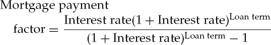
Note that the interest rate in question is the monthly rate, that is, the annual percentage rate divided by 12. The monthly payment is then computed by multiplying the mortgage payment factor by the loan's balance (either original or, if the loan is being recast, the current balance).
As an example, consider the following loan:
Loan balance: | $100,000 |
Annual rate: | 6.0% |
Monthly rate: | 0.50% = 0.005 |
Loan term: | 30 Years (360 Months) |
The monthly payment factor is calculated as
Therefore, the monthly payment on the subject loan is $100,000 × 0.0059955, or $599.55.
An examination of the allocation of principal and interest over time provides insights with respect to the buildup of owner equity. As an example, Figure 18.1 shows the total payment and the amount of principal and interest for the $100,000 loan with a 6.0% interest rate (or note rate, as it is often called) for the life of the loan.
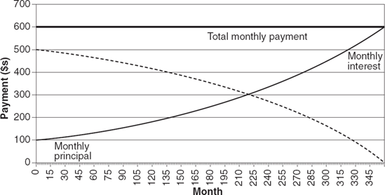
Figure 18.1. Monthly Payment Breakdown for a $100,000 Fixed-Rate Loan at 6.0% Rate with a 30-Year Term (fixed payment of $599.55 per month)
The exhibit shows that the payment is comprised mostly of interest in the early period of the loan. Since interest is calculated from a progressively declining balance, the amount of interest paid declines over time. In this calculation, since the aggregate payment is fixed, the principal component consequently increases over time. In fact, the exhibit shows that the unpaid principal balance in month 60 is $93,054, which means that only $6,946 of the $35,973 in payments made by the borrower up to that point in time consisted of principal. However, as the loan seasons, the payment is increasingly allocated to principal. The crossover point in the example (that is, where the principal and interest components of the payment are equal) for this loan occurs in month 222.
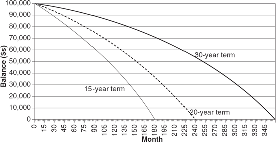
Loans with shorter amortization schedules (e.g., 15-year loans) allow for buildup of equity at a much faster rate. Figure 18.2 shows the outstanding balance of a $100,000 loan with a 6.0% note rate using 30-, 20-, and 15-year amortization terms. In contrast to the $93,054 remaining balance on the 30-year loan, the remaining balances on 20- and 15-year loan in month 60 are $84,899 and $76,008, respectively. In LTV terms, if the purchase price of the home is $125,000 (creating an initial LTV of 80%), the LTV in month 60 on the 15-year loan is 61% (versus 74% for the 30-year loan). Finally, while 50% of the 30-year loan balance is paid off in month 252, the halfway mark is reached in month 154 with a 20-year term, and month 110 for a 15-year loan.
Patterns of borrower equity accumulation due to amortization are important in understanding the attributes of interest-only loans. Figure 18.3 compares the remaining balances over time for the previously described fully amortizing $100,000 loan with a 6% rate, versus an interest-only loan with the same rate and term. A fully amortizing loan would have a monthly payment of $599.95, and would have reduced its principal balance by $6,946 at the end of five years. The interest-only loan, by definition, would amortize none of the principal over the same period. It would have an initial monthly payment at the 6% rate of $500, which would increase to $644 when the loan recasts in month 60. The 29% increase in the payment results from the loan's balance being amortized over the remaining term of 300 months. As Figure 18.3 indicates, the remaining balance of the interest-only loan amortizes faster than the fully amortizing loan because of the higher payment, although the interest-only loan's remaining balance is greater than that of the amortizing loan. The LTV of the amortizing loan (assuming a purchase price of $125,000 and an original LTV of 80%) declines to roughly 74% by month 60 and 72% in month 80. The interest-only loan has an 80% LTV through the first 60 months after issuance, but by month 80 the LTV declines to 77.5%.
For amortizing ARM loans, the initial payment is calculated at the initial note rate for the full 360-month term. At the first reset, and at every subsequent adjustment, the loan is recast, and the monthly payment schedule is recalculated using the new note rate and the remaining term of the loan. For example, payments on a five-year hybrid ARM with a 5.5% note rate would initially be calculated as a 5.5% loan with a 360-month term. If the loan resets to a 6.5% rate after five years (based on both the underlying index and the loan's margin), the payment is calculated using a 6.5% note rate, the remaining balance in month 60, and a 300-month term. In the following year, the payment would be recalculated again using the remaining balance and prevailing rate (depending on the performance of the index referenced by the loan) and a 288-month term. In this case, the loan's initial monthly payment would be $568; in month 60, the loan's payment would change to $624, or the payment at a 6.5% rate for 300 months on a $92,460 remaining balance. (Note that all rate changes are subject to caps that limit the amount that the rate can change over a designated period of time.)
The payments on an interest-only hybrid ARM are similar to those of a fixed rate, interest-only loan. Using the rate structure described above, an interest-only 5/1 hybrid ARM would have an initial payment of $458. After the 60-month fixed rate, interest-only period, the monthly payments would reset at $675, an increase of roughly 47%. This increase represents the payment shock discussed previously. Depending on the loan's margin and the level of the reference index, borrowers seeking to avoid a sharp increase in monthly payments often refinance their loans into cheaper available products. The desire to mitigate payment shock is also largely responsible for the growth in hybrid ARMs with noncontiguous resets. Since these loans essentially separate the rate reset and payment recast, the payment increases are spread over two periods, reducing the impact of a large one-time increase in payment.
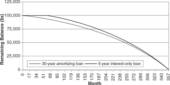
Figure 18.3. Remaining Principal Balance Outstanding for $ 100,000 6% Loan, Fully Amortizing versus Five-Year Interest-Only Loans
The payment structure for negative-amortization ARM loans is different and complex. The most commonly issued form of products that allow negative amortization are so-called payment-option loans, which incorporate the features of a number of different ARM products. The loans have an introductory rate that is effective for a short period of time (either one or three months). After the initial period, the loan's rate changes monthly, based on changes in the reference index. The borrower's minimum or "required" payment, however, does not change until month 13. The initial or teaser payment is initially calculated to fully amortize the loan over 30 years at the introductory rate. After a year, and in one-year intervals thereafter, the loan is recast. The minimum payment is recalculated based on the loan's margin, the index level effective at that time, and the remaining balance and term on the loan. However, the increase in the loan's minimum monthly payment is subject to a 7.5% cap. (Note that this cap functions differently than those in the hybrid market, which are based on changes in the loan's rate rather than payment.)
The minimum payment may not be sufficient to fully pay the loan's interest, based on its effective rate. This may occur if the loan's index and margin are such that the minimum payment is lower than the interest payment, or if the minimum payment is constrained by the 7.5% payment cap. In that event, the loan undergoes negative amortization, where the unpaid or "deferred" amount of interest is added to the principal balance. Negative amortization is typically limited to 115% of the original loan balance (or 110% in a few states). If this threshold is reached, the loan is immediately recast to amortize the current principal amount over the remaining term of the loan. Under all circumstances, the loan is automatically recast periodically, with payments calculated based on the current loan balance and the remaining term of the loan. At this point, the payment change is not subject to the 7.5% payment cap—a condition that also holds true if the loan recasts because the negative amortization cap is reached. (The first mandatory recast is generally at the beginning of either year 5 or 10; in either case, the loan will subsequently recast every five years thereafter.)
Holders of fixed income investments ordinarily deal with interest rate risk, or the risk that changes in the level of market interest rates will cause fluctuations in the market value of such investments. However, mortgages and associated mortgage products have additional risks associated with them that are unique to the products and require additional analysis. We conclude this chapter with a discussion of these risks.
In a previous section, we noted that obligors have the ability to prepay their loans before they mature. For the holder of the mortgage asset, the borrower's prepayment option creates a unique form of risk. In cases where the obligor refinances the loan in order to capitalize on a drop in market rates, the investor has a high-yielding asset pay off, and it can be replaced only with an asset carrying a lower yield. Prepayment risk is analogous to "call risk" for corporate and municipal bonds in terms of its impact on returns, and also creates uncertainty with respect to the timing of investors' cash flows. In addition, changing prepayment "speeds" due to interest rate moves cause variations in the cash flows of mortgages and securities collateralized by mortgage products, strongly influencing their relative performance and making them difficult and expensive to hedge.
Prepayments are phenomena resulting from decisions made by the borrower and/or the lender, and occur for the following reasons:
The sale of the property (due to normal mobility, as well as death and divorce).
The destruction of the property by fire or other disaster.
A default on the part of the borrower (net of losses).
Curtailments (that is, partial prepayments).
Refinancing.
Prepayments attributable to reasons other than refinancings are referred to under the broad rubric of "turnover." Turnover rates tend to be fairly stable over time, but are strongly influenced by the health of the housing market, specifically the levels of real estate appreciation and the volume of existing home sales. Refinancing activity, however, generally depends on being able to obtain a new loan with either a lower rate or a smaller payment, making this activity highly dependent on the level of interest rates, the shape of the yield curve (since short rates strongly influence ARM pricing), and the availability of alternative loan products. In addition, the amount of refinancing activity can change greatly as the result of seemingly small changes in rates.
The paradigm in mortgages is thus fairly straightforward. Mortgages with low note rates (that are "out-of-the-money," to borrow a term from the option market) normally prepay fairly slowly and steadily, while loans carrying higher rates (and are "in-the-money") are prone to experience spikes in prepayments when rates decline. Clearly, this paradigm is dependent on the level of mortgage rates.
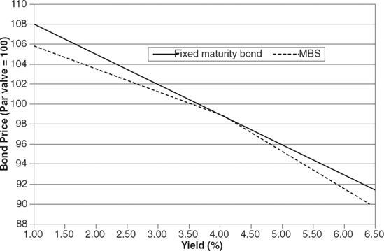
It is important to understand how changes in prepayment rates impact the performance of mortgages and MBS. Since prepayments increase as bond prices rise and market yields are declining, mortgages shorten in average life and duration when the bond markets rally, constraining their price appreciation. Conversely, rising yields cause prepayments to slow and bond durations to extend, resulting in a greater drop in price than experienced by more traditional (that is, option-free) fixed income products. As a result, the price performance of mortgages and MBS tends to lag that of comparable fixed maturity instruments (such as Treasury notes) when the prevailing level of yields increases.
This phenomenon is generically described as negative convexity. The effect of changing prepayment speeds on mortgage durations, based on movements in interest rates, is precisely the opposite of what a bondholder would desire. (Fixed income portfolio managers, for example, extend durations as rates decline, and shorten them when rates rise.) The price performance of mortgages and MBS is, therefore, decidedly nonlinear in nature, and the product will underperf orm assets that do not exhibit negatively convex behavior as rates decline.
Figure 18.4 shows a graphic representation of this behavior. Investors are generally compensated for the lagging price performance of MBS through higher base-case yields. However, the necessity of managing negative convexity and prepayment risk on the part of investors involves fairly active management of MBS portfolios, and creates both higher hedging costs and the possibility of losses due to estimation and modeling error. In turn, this creates the desire on the part of some investors to limit their exposure to prepayments by investing in bonds where prepayment risk is transferred within the structure. This type of risk mitigation is central to the structured MBS market.
Analysis of the credit exposure in the mortgage sector is different from the assessment of credit risk in most other fixed income instruments because it requires:
Quantifying and stratifying the characteristics of the thousands of loans that underlie the mortgage investment.
Estimating how these attributes will translate into performance based on standard metrics, and the evaluation of reasonable best-, worst-, and likely-case performance.
Calculating returns based on these scenarios.
In a prior section, some of the factors (credit scores, LTVs, etc.) that are used to gauge the creditworthiness of borrowers and the likelihood of a loan to result in a loss of principal were discussed. Many of the same measures are also used in evaluating the creditworthiness of a mortgage pool. For example, weighted average credit scores and LTVs are routinely calculated, and stratifications of these characteristics (along with documentation styles and other attributes) are used in the credit evaluation of the pool. In addition to these characteristics of the loans, the following metrics are also utilized in the a posteriori evaluation of a mortgage pool or security.
Delinquencies
These measures are designed to gauge whether borrowers are current on their loan payments or, if they are late, stratifying them according to the seriousness of the delinquency. The most common convention for classifying delinquencies is one promulgated by the Office of Thrift Supervision; this "OTS" method classifies loans as follows:
Payment due date to 30 days late: Current
30–60 days late: 30 days delinquent
60–90 days late: 60 days delinquent
More than 90 days late: 90+ days delinquent
Defaults
At some point in their existence, many loans that are associated with delinquencies become current or "cure," as the condition leading to the delinquency (e.g., job loss, illness, etc.) resolves itself. However, some portion of the delinquent loan universe ends up in default. By definition, default is the point where the borrower loses title to the property in question. Default generally occurs for loans that are 90+ days delinquent, although loans where the borrower goes into bankruptcy may be classified as defaulted at an earlier point in time.
Loss Severity
Since the lender has a lien on the borrower's property, much of the value of the loan can be recovered through the foreclosure process. Loss severity measures the face value of the loss on a loan after foreclosure is completed. Depending on the type of loan, loss severities can average in the area of 20% to 40%, and can be heavily influenced by the loan's LTV (since a high LTV loan leaves less room for a decline in the value of the property in the event of a loss). However, in the event of a default, loans with relatively low LTVs can also result in losses, generally for two reasons:
The appraised value of the property may be high relative to the property's actual market value.
There are costs and foregone income associated with the foreclosure process.
In light of these factors, the process of evaluating the credit-adjusted performance of either a group of loans involves first gauging the expected delinquencies, defaults, and loss severities of the pool or security based on its credit characteristics. Subsequently, loss-adjusted yields and returns can be generated. It should be noted that investors in some segments of the MBS market do not engage in detailed credit analysis; buyers of agency pools, for example, generally rely on the guaranty of the agency in question. In addition to buyers of mortgages in whole-loan form, credit analysis is primarily undertaken by investors in the subordinate tranches of private label deals. As one might expect, the performance of subordinates is highly sensitive to the credit performance of the collateral pool. This is both because of their role in protecting the senior classes from losses, as well as the sequential nature of loss allocations within the subordinate classes.
Mortgage products can be defined by a number of critical attributes. These include lien status, loan term, credit classification, interest rate type, and amortization scheme. Many loan products are based on a mix of attributes; an example might be an adjustable-rate loan with an interest-only feature. Loans can be securitized either by using the guarantees of a government agency or quasi-governmental entity (that is, the GSEs), or by utilizing a so-called private-label structure that incorporates credit enhancement through mechanisms such as subordination. An important characteristic defining loans refers to their interest rate classification. Fixed-rate loans have an interest rate fixed for the life of the loan, while adjustable-rate mortgages (or ARMs) reset periodically to a rate based on a reference index. The borrower's payment on an ARM will typically change at the reset date. Depending on the shape of the yield curve and the level of the index, the rate may increase or decrease. An increased payment may create a "payment shock" in which the borrower's payment increases significantly over its initial level.
Mortgage loans have traditionally been issued as fully-amortizing obligations with (for fixed-rate products) a constant payment over their term. However, loans with alternative payment schemes (such as interest-only loans) have become increasingly popular. When the interest-only lockout expires, loans structured as interest-only products will recast in order to amortize the loan over the remaining term. This event creates another form of payment shock, and for interest-only ARMs will exacerbate the payment shock experienced at the reset date. Mortgage loans and mortgage-backed securities have fairly unique risk profiles. Their performance can suffer from changes in prepayment speeds (creating "negative convexity") as well as, for loans in raw form and subordinated MBS, exposure to credit risk.
Bhattacharya, A. K., Berliner, W. S., and Lieber, J. (2006). Alt-A mortgages and MBS. In E J. Fabozzi (ed.), Handbook of Mortgage-Backed Securities, 6th edition. New York: McGraw-Hill, pp. 187−206.
Bhattacharya, A. K., Banerjee, S., Horowicz, R., and Wang, W (2006). Hybrid adjustable-rate mortgages (ARMs). In E J. Fabozzi (ed.), Handbook of Mortgage-Backed Securities, 6th edition (pp. 259-286). New York: McGraw-Hill.
Fabozzi, E J. (ed.) (2006). Handbook of Mortgage-Backed Securities, 6th edition. New York: McGraw-Hill.
Fabozzi, E J. (2006). Fixed Income Mathematics: Analytical and Statistical Techniques, 4th edition. New York: McGraw-Hill Publishing.
Fabozzi, E J., Bhattacharya, A. K., and Berliner, W S. (2007). Mortgage-Backed Securities: Products, Structuring, and Analytical Techniques. Hoboken, NJ: John Wiley & Sons.
Fabozzi, E J., and Modigliani, E (1992). Mortgage and Mortgage-Backed Securities Markets. Boston: Harvard Business School Press.
Liu, D. (2006). Interest-only ARMs. In E J. Fabozzi. (ed.), Handbook of Mortgage-Backed Securities, 6th edition (pp. 333-362). New York: McGraw-Hill.
Mansukhani, S. (2006). Exploring the MBS/ABS continuum: The growth and tiering of the Alt-A hybrid sector. In E J. Fabozzi (ed.), Handbook of Mortgage-Backed Securities, 6th edition (pp. 171-186). New York: McGraw-Hill.
Mansukhani, S., Budhram, A., and Qubbaj, M. (2006). Fixed-rate Alt-A MBS. In E J. Fabozzi. (ed.), Handbook of Mortgage-Backed Securities, 6th edition (pp. 207-258). New York: McGraw-Hill.