ROBERT WHALEY, PhD
Valere Blair Potter Professor of Management, The Owen Graduate School of Management, Vanderbilt University
Abstract: A relatively new stock index product is the volatility derivative. The Chicago Board Options Exchange (CBOE) contemplated launching trading volatility options as early as 1993. On January 19, 1998, the Deutsche Terminborse (DTB) became the first exchange in the world to list volatility futures. The CBOE launched trading of VIX futures on its CBOE Futures Exchange on March 26, 2004, with contracts on three-month realized variance being launched on May 18, 2004. The CBOE launched VIX options on February 24, 2006. It was not until the Long-Term Capital Management (LTCM) fiasco in late 1998 that the market finally began to recognize the value of trading stock market volatility as a separate asset class.
Keywords: volatility derivatives, volatility swap, realized future volatility, realized volatility derivative contract, variance swap, implied volatility derivatives contract
Volatility derivative contracts are written not only on stock indexes, but also interest rates, currencies, and commodities like crude oil. Prior to the advent of volatility derivatives, stock market volatility risk was managed using options written on the underlying index. The problem with doing so is that it is expensive. Options have two sources of price risk—risk associated with movements in the underlying index level and risk associated with movements in the market's perception of expected future volatility rate. The only way to isolate the volatility exposure is by trading the options and delta-hedging using the underlying index, index futures, and other index options.
This chapter describes volatility derivative contracts and their uses. We focus primarily on stock market volatility since stock market volatility contracts are the most actively traded. The discussion has two parts. First, we discuss realized volatility contracts and their applications, and then we turn to implied volatility contracts.
At the outset, we need to correct a misnomer. Industry has come to refer to realized volatility contracts as volatility swaps. A volatility swap is not a swap; it is a forward contract. They have traded in OTC markets for more than five years, and are now also exchange traded.
A volatility forward (or swap) is written on the realized future volatility of an asset (say, the S&P 500 index). At expiration, its payoff is based on the statistical formula for the annualized standard deviation of index return, that is, where nT is the number of price observations used in the computation, and St is the index level.
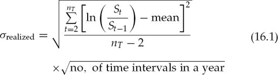
Volatility forwards are usually based on daily closing prices, however, since they are traded primarily in the OTC market, any frequency (e.g., hourly, weekly) is possible. The contract also specifies the source from which for the prices will be obtained. Volatility forwards are sometimes based on squared returns, and sometimes on squared deviations. Formula (16.1) shows squared deviations. The formula for squared returns is the special case where the mean term in the squared brackets of (16.1) is set equal to zero and the adjustment in the numerator is increased to nT −1. Finally, the volatility is annualized. For daily prices, the last term on the right-hand side is usually
The value represented by formula (16.1) is the price of the asset underlying the forward contract at expiration. The only difference is the underlying asset is not tradable; it is simply a computation of realized volatility. At inception, the buyer and seller agree to a fixed delivery price (quoted as an annualized volatility), σX, on the expiration date, T. As expiration approaches, the forward's settlement price becomes more and more certain because some of the prices used in (16.1) have been realized already. On the last day before expiration, only the index level on expiration day remains unknown. Upon settlement, the buyer receives
that is, the notional amount of the swap times the difference between the realized and contracted volatility. The seller receives the opposite amount. Sometimes the volatility derivatives are written on the square of volatility, or variance. The buyer of a variance swap receives the payoff,
Suppose that on Friday, August 1, 2003, an investor bought a 13-week volatility forward from an OTC derivatives dealer. Its price was 0.12, and its notional amount was $100 million. The Friday closing index levels over the period were as follows:
Friday Close | S&P 500 Index |
|---|---|
20030801 | 980.15 |
20030808 | 977.59 |
20030815 | 990.67 |
20030822 | 993.06 |
20030829 | 1008.01 |
20030905 | 1021.39 |
20030912 | 1018.63 |
20030919 | 1036.30 |
20030926 | 996.85 |
20031003 | 1029.85 |
20031010 | 1038.06 |
20031017 | 1039.32 |
20031024 | 1028.91 |
20031031 | 1050.71 |
The first step in calculating the settlement price and settlement proceeds is to compute the weekly returns. Next compute the mean weekly return, and the squared returns and deviations. Compute the sum of squares and the annualized volatility. To annualize weekly returns, use the factor,
Table 16.1. Computations for Settlement Price and Settlement Proceeds for a Realized Volatility Swap
Friday Close | S&P 500 Index | S&P 500 Return | Squared Returns | Squared Deviations |
|---|---|---|---|---|
20030801 | 980.15 | |||
20030808 | 977.59 | −0.00262 | 0.00000684 | 0.00006340 |
20030815 | 990.67 | 0.01329 | 0.00017665 | 0.00006310 |
20030822 | 993.06 | 0.00241 | 0.00000581 | 0.00000863 |
20030829 | 1008.01 | 0.01494 | 0.00022327 | 0.00009206 |
20030905 | 1021.39 | 0.01319 | 0.00017388 | 0.00006145 |
20030912 | 1018.63 | −0.00271 | 0.00000732 | 0.00006485 |
20030919 | 1036.30 | 0.01720 | 0.00029577 | 0.00014044 |
20030926 | 996.85 | −0.03881 | 0.00150634 | 0.00195002 |
20031003 | 1029.85 | 0.03257 | 0.00106068 | 0.00074097 |
20031010 | 1038.06 | 0.00794 | 0.00006305 | 0.00000672 |
20031017 | 1039.32 | 0.00121 | 0.00000147 | 0.00001709 |
20031024 | 1028.91 | −0.01007 | 0.00010134 | 0.00023759 |
20031031 | 1050.71 | 0.02097 | 0.00043958 | 0.00024395 |
Mean | 0.00535 | |||
Total | 0.00033850 | 0.00030752 | ||
Annualized volatility | 0.13267 | 0.12646 | ||
Notional amount | $100,000,000 | $100,000,000 | ||
Forward price | 0.120 | 0.120 | ||
Cash settlement value | $1,267,275 | $645,649 |
Table 16.2. Selected Terms of S&P 500 Three-Month Variance Future Contract
Exchange | CBOE Futures Exchange (CFE) |
Ticker symbol | VT |
Contract unit | $50 per variance point |
Tick size | 0.5 of one variance point |
Tick value | $25 |
Trading hours | 8:30 AM to 3:15 PM CST |
Contract months | Up to four contract months on the March cycle (Mar., Jun., Sep., Dec.) |
Last day of trading | Close of trading on business day before final settlement date. |
Final settlement date | Third Friday of contract month. |
Final settlement price | Final settlement price is based on the standardized calculation of the realized variance of the S&P 500. |
This calculation uses continuously compounded daily returns for a three-month period assuming a mean daily return of zero. The calculated variance is then annualized assuming 252 business days per year. The final settlement price is this annualized, calculated variance multiplied by 10,000. |
The CBOE Futures Exchange (CFE) launched its three-month realized volatility futures contract on May 18, 2004. The CFE is an all-electronic exchange that was created by the Chicago Board Options Exchange (CBOE) in March 2004. The CFE's realized volatility contract is based on S&P 500 return variance rather than return standard deviation, and its product specifications are provided in Table 16.2 The contract denomination is $50 per variance point. A price quotation of 633.50, for example, means the contract value is $31,675. Up to four contracts may trade simultaneously. The contracts are on the March quarterly expiration cycle (March, June, September, December). The final settlement date is the third Friday of the contract month. Trading stops at the close on the preceding business day.
The final settlement price is a variance number and assumes the mean return is zero. Hence, the realized volatility formula (16.1) becomes
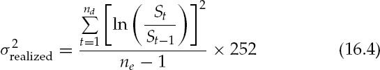
where na is the actual number of trading days in the three-month interval, and ne is the expected number of days in the three-month interval. Normally, na and ne are equal. In the event of a market disruption during the contract's life, however, na will be less than ne. Generally speaking, a "market disruption event," as determined by the CFE, occurs when trading on the primary exchanges of a significant number of S&P 500 stocks is suspended or limited in some way or when the primary exchange on which index stocks unexpectedly closes early (or does not open) on a particular day. For each market disruption event, the value of na is reduced by one.
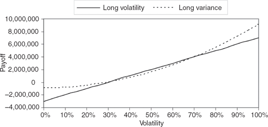
The industry has come to define volatility as the standard deviation of the natural logarithm of the price ratios (This is consistent with the Black-Scholes model's use of continuously compounded returns). If the forward is defined in terms of variance (that is, volatility squared) rather than volatility, the payoff structure is quite different. Consider Figures 16.1 and 16.2 which plot the payoffs of a volatility forward contract versus a variance forward contract for long and short positions. Since the horizontal axis is defined in terms of volatility, its terminal payoffs are a linear function of volatility. The variance forward, however, is nonlinear. The long variance position (the dotted line in Figure 16.1) has convexity. As volatility falls, the terminal payoff of the long variance position decreases, but at a decreasing rate. At the same time, as volatility increases, the terminal payoff of the long variance forward increases at an increasing rate. Indeed, the variance payoffs loosely resemble a long call position, while the variance payoffs of the short variance futures resemble a short call position.
At first blush, the volatility forward contract seems to be purely a speculative instrument. Traders who believe future volatility will be high relative to the forward price will go long the swap, and those who believe that the market will be very calm will go short. But, the hedging possibilities using realized volatility forwards are many. In the normal course of operation, for example, some market participants become inherently short volatility. Consider the ill-fated index option strategy of Long-Term Capital Management (LTCM). Because index option implied volatilities were as high as they had been anytime since the October 1987 market crash, LTCM sold both index calls and puts with the belief that implied volatility would return to normal levels. Unfortunately, a problem arose when implied volatility continued to rise and their positions were marked-to-market. The cash drain was enormous. Buying realized volatility forwards would have hedged this exposure, at least in part. The same is true for index option market makers who are short market volatility as a result of selling index puts to portfolio insurers (On a typical day. S&P 500 put option volume (and open interest) is nearly double that of S&P 500 calls).
Another hedging possibility is for risk arbitrageurs. Immediately after a merger is announced, risk arbitrageurs step in and buy shares of a target firm and sell the shares of bidder. Because the probability that the merger will be successful is not known, the prices of the target and the bidder will not fully reflect the terms of the offer. If the merger is successful, the spread between the prices will converge. Before the deal is consummated, however, market volatility may increase, making the merger less likely, thereby causing the spread to widen. Buying a realized volatility forward contract can hedge this type of risk exposure.
Yet another application is for individuals or portfolio managers who attempt to track some sort of benchmark index. During periods of high volatility, the portfolio may require more frequent rebalancing and greater transaction cost expenses. Again, buying a realized forward contract on volatility can hedge this exposure.
The CFE also lists a futures contract written on the implied return volatility of the S&P 500 index. The CBOE Marker Volatility Index or VIX is constructed in such a way that it represents the implied volatility of an at the money S&P 500 index option with exactly thirty calendar days to expiration. It is sometimes called the "investor fear gauge" because it is set by investors and expresses their consensus view about expected future stock market volatility. The specific details of its construction are contained in appendix to this chapter. What is interesting about its construction is that the index can be created using a static portfolio of SPX options. This is important since arbitrage between the VIX futures and the underlying VIX index promotes liquidity in both markets.
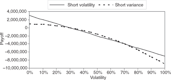
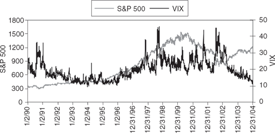
Figure 16.3. Daily Levels of the S&P 500 Index and the VIX during the Period January 1990 through December 2004
The relation between the movements of the VIX and the movements of the S&P 500 index are important to understand. Figure 16.3 shows the daily levels of the S&P 500 index and the VIX during the period January 1990 through December 2004. A number of interesting patterns appear.
First, note that the VIX level (that is, the dark line) is more jagged than the S&P 500 index level. What this means is that the volatility of the volatility of the S&P 500 index is greater than the volatility of the index itself. Time-series variation in the expected volatility of stock indexes has been documented in a number of studies. Day and Lewis (1992), for example, demonstrate that the expected variance of the S&P 100 index follows a mean-reverting process. They also show that implied volatilities from S&P 100 index options (OEX) explain a significant amount of the changes in expected variance. In a related paper, Fleming (1998) finds that OEX implied volatilities are good (but not perfect) forecasts of future volatility.
Second, there tends to be an inverse relation between the level of VIX and the level of the S&P 500 index—as the stock market goes up, volatility tends to fall. During 2003 and 2004, for example, the S&P 500 is systematically increasing while the level of VIX falls. Third, the inverse correlation is not perfect. During 1996 and 1997, for example, the level of market volatility is increasing while the stock market is also increasing. All of these phenomenon contribute to making futures contracts on the VIX a potentially new and useful expected return/risk management tool, as we will see in the illustration that follows.
The CFE VIX futures contract has, as its underlying, the VIX. The futures contract specifications are given in Table 16.3. Its denomination is $100 times the increased-value VIX. The "increased-value VIX" (ticker symbol VBI) is simply the level observed in the marketplace times ten (VBI = VIX × 10). The tick size of the contract is 0.1 of one VBI point or $10. The available contract months include the two near-term contract months plus two contract months on the February quarterly cycle (February, May, August, and November). The expiration day is the third Friday of the contract month, although trading stops on the preceding Tuesday. The contract is cash-settled on the Wednesday preceding the third Friday, at a special opening quotation (SOQ).
Table 16.3. Selected Terms of Market Volatility Index (VIX) Futures Contract
| [a] | |
|---|---|
Exchange | CBOE Futures Exchange (CFE) |
Ticker symbol | VX |
Contract unit | $100 times Increased-Value VIX[a] |
Tick size | 0.1 of one VBI point |
Tick value | $10 |
Trading hours | 8:30 AM to 3:15 PM CST |
Contract months | Two near-term contract months plus two contract months on the February quarterly cycle (Feb., May, Aug., and Nov.) |
Expiration day | Third Friday of the contract month. |
Last day of trading | Tuesday prior to the third Friday of the expiring month. |
Final settlement date | Wednesday prior to the third Friday of the expiring month. |
Final settlement price | Cash settled. Final settlement price for VIX futures shall be 10 times a Special Opening Quotation (SOQ) of VIX calculated from the options used to calculate the index on the settlement date. The opening price for any series in which there is no trade shall be the average of that option's bid price and ask price as determined at the opening of trading. The final settlement price will be rounded to the nearest 0.10. |
[a] Increased-Value VIX (VBI) is 10 times the VIX index level. | |
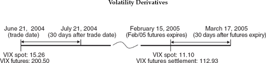
To understand the distinction between the VIX and the VIX futures, consider Figure 16.4. The figure assumes that we traded the February 2005 VIX futures on June 21, 2004. At the close on June 21, the VIX level was 15.26, and the Feb/05 VIX was at 200.50. Recall that the futures is scaled by 10, so the futures price represents a volatility rate of 20.05%. As the figure illustrates, the level of VIX reflects the market's expected future volatility over the next thirty calendar days (from June 21 to July 21, 2004), while the VIX futures reflects the expected future market volatility during a 30-calendar day period beginning when the Feb/05 futures contract expires and ending 30 calendar days later (February 15 to March 17, 2005). In other words, the VIX futures is a one-month forward volatility rate that begins some time in the future. As it turns out, on February 15, 2005, the Feb/05 VIX was cash settled in the morning at ten times the spot level of VIX, 112.93. By the end of the day, the level of VIX had fallen to 11.10.
The convergence of the Feb/05 VIX futures to the VIX index over the period June 21, 2004 through February 15, 2005 is shown in Figure 16.5. The VIX is multiplied by 10 to put it on the same scale as the futures price. Where the two prices were about 50 points apart in June 2004, they slowly and steadily converged to the same level at expiration. Figure 16.6 shows the open interest of the Feb/05 VIX futures contract. In June 2004, the Feb/05 futures was a distant contract maturity and did not have much open interest. Through time, as the shorter contract maturities expired, the open interest in the Feb/05 contract rose, reaching a peak above 6,000 contracts in January 2005. Like most cash-settled futures, open interest remained high until contract settlement (Futures contracts with physical delivery are generally unwound before contract maturity to avoid the costs of transportation. With cash settlement, no such costs exist.)
To get a sense for how VIX futures contracts are priced, let us assume that we are considering the variance of S&P 500 index returns over the next 60 calendar days (that is, two months). If the returns of the index are independent through time, we can write
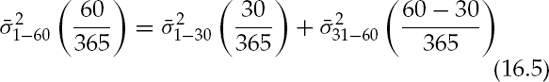
In (16.5), σ−21−60 and σ−21−60 can be considered spot rates of variance, that is, the expected variance rates over the next 30 calendar days and 60 calendar days, respectively. The term,
however, is a forward variance, that is, the average variance rate that we can expect to observe over a 30-day period beginning 30 days from now. To determine the forward volatility rate, we can rearrange (16.5) to yield
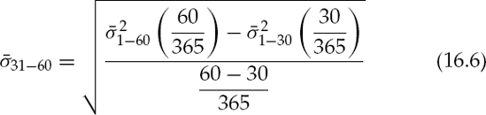
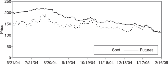
Figure 16.5. Convergence of February 2005 VIX Futures Price to VIX Spot Price (10 times observed VIX) over the Period June 21, 2004, through February 16, 2005
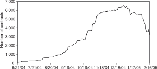
Figure 16.6. Open Interest of February 2005 VIX Futures over Its Life (June 21, 2004, through February 16, 2005).
Equation (16.6) provides us with the insight we need in understanding how to value the VIX futures. The rate on the left-hand side of (16.6) can be thought of as the VIX futures price. In order to estimate its value, we need to know the two variance rates in the numerator on the right-hand side. One way to get these values is to request quotes on 30-day and 60-day variance forwards from an OTC swap dealer. Another is to use S&P 500 index options to imply the variance rates of 30- and 60-day intervals. Note that, in this particular instance, the rate
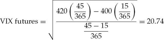
Suppose that an investor is given the assignment of determining the fair value of the VIX futures where the contract expires in exactly 15 days. The investor has contacted an OTC derivatives dealer, and the dealer quoted the investor rates of 400 and 420 on 15-day and 45-day realized variance swaps.
The quoted realized variance swap rates straddle the forward period corresponding to the VIX futures. Hence, the fair value of the VIX futures can be determined by expressed in VIX points, or 207.40 expressed in VBI points.
Exchange-traded futures on volatility also offer a number of new expected return/risk management strategies. VIX futures can be regarded as a new asset class and can potentially improve the expected return/risk opportunity set. Indeed, because the returns of the S&P 500 portfolio and the returns of the VIX are inversely correlated, the diversification effects can well surpass other strategies such as diversifying across countries (Stock returns in different countries tend to be positively correlated. A major economic shock in one market is usually felt across markets.) VIX futures can also be used to manage individual stock volatility. Individual stock volatility can be thought of as the sum of two components: stock market volatility and firm-specific volatility. Market volatility products allow investors to hedge the stock market volatility component to develop selected exposures in the idiosyncratic risk of individual stocks (Whaley [1993] demonstrates that, for large market capitalizaton firms, nearly 50% of movement in individual stock volatility rate is explained by movements in the market volatility rate.)
One caveat is necessary, however. Many stock market volatility hedging needs are long term. The VIX futures contract, however, is on the stock market volatility rate in a 30 day forward period. Consequently, in order to effectively hedge a short volatility position over a long period of time, it may be necessary to buy a strip of VIX futures so that the volatility rate over the entire hedge interval may be captured.
The Chicago Board Options Exchange (CBOE) launched VIX option contracts on Friday, February 24, 2006. Like the VIX futures, the CBOE's VIX options contract has, as its underlying, the VIX. The option contract specifications are given in Table 16.4. Its ticker symbol is "VIX," and its denomination is $100 times the level of the CBOE's
Table 16.4. Selected Terms of Market Volatility Index (VIX) Option Contract
Exchange | Chicago Board Options Exchange (CBOE) |
Ticker symbol | VIX |
Contract unit | 100 times CBOE Market Volatility index |
Exercise price increments | 2-1/2 point increments |
Exercise style | European |
Tick size | 0.05 point up to $3 premiums; 10 point over $3 |
Tick value | $5; $10 |
Trading hours | 8:30 AM to 15:15 PM CST |
Contract months | Two near-term contract months plus two contract months on the February quarterly cycle (Feb., May, Aug., and Nov.) |
Expiration day | Wednesday that is 30 days prior to the third Friday of the calendar month immediately following the expiring month. |
Last day of trading | Tuesday prior to expiration date each month. |
Final settlement price | Cash settled. Exercise settlement value shall be a Special Opening Quotation (SOQ) of VIX calculated from the sequence of opening prices of options used to calculate the index on the settlement date. The opening price for any series in which there is no trade shall be the average of that option's bid price and ask price as determined at the opening of trading. Exercise will result in the delivery of cash on the business day following expiration. The exercise settlement amount is equal to the difference between the exercise-settlement value and the exercise price of the option times $100. |
Market Volatility index. The tick size (value) of the contract is 0.05 ($5) for option premiums below $3.00 ($300), and 0.10 ($100) for premiums greater than $3 ($300). The available contract months include the two near-term contract months plus two contract months on the February quarterly cycle (February, May, August, and November). The expiration day is the Wednesday that is 30 days before the third Friday of the calendar month following the expiring month. Trading stops on the Tuesday before the expiration day. The contract is cash-settled on the day after the expiration at a special opening quotation (SOQ). The exercise settlement amount equals the difference between the exercise-settlement value and the exercise price times $100.
There are two types of volatility derivative contracts—contracts on realized volatility and contracts on volatility implied by index option prices. In this chapter we describe the different volatility contract specifications and explain how the CBOE's Market Volatility Index (VIX) can be constructed from a portfolio of S&P 500 index options. We also note that volatility derivatives can be used as an alternative investment in an asset allocation framework.
The purpose of this appendix is to describe the algorithm with which the CBOE's Market Volatility Index (VIX) is computed.
The procedure for calculating VIX is described in CBOE (2003). The theory underlying the procedure is based on the Breeden and Litzenberger (1978) result that the probability density function of asset price can be inferred from the prices of options written on that asset, where the options have a common expiration date and continuum of exercise prices. Demeterfi, Derman, Kamal, and Zou (1999) apply this result in a discretized form to arrive at an equation for the volatility of asset price.
The VIX is the expected future volatility of the S&P 500 index over the next 30 days. It is an implied volatility in that it is based on S&P 500 index option prices. Unlike the implied volatilities from the Black-Scholes-Merton (BSM) option valuation model, however, the VIX does not depend on a particular return distribution (The BSM model assumes a log-normal asset price distribution at the option's expiration.)
To compute the VIX, an eight-step procedure is used.
Step 1: Collect relevant information. The information needed to compute the VIX is (1) the bid/ask price quotes of all nearby and second nearby call and put options traded on the S&P 500 index; and (2) the risk-free interest rate corresponding to each expiration date. For each option series, the bid/ask midpoint is computed. The difference between the call midpoint and put midpoint at each exercise price is computed.
Step 2: Compare the time to expiration in minutes and then years from the current time until option expiration. The time to expiration in minutes is the sum of three components (Time to expiration is computed in minutes to conform to industry practice.) First, we must compute the number of minutes from the current time until midnight on the same day. We next compute the number of minutes from midnight today until midnight on the day before expiration. Finally, we must compute the number of minutes from midnight on the day before expiration until cash settlement at the open on expiration day. The last number is, of course, a constant. The time of cash settlement is at 8:30 AM on expiration day. The number of minutes from midnight on the day before expiration until the time of expiration is therefore
The first and second components depend upon the time of day and the number of days to expiration, respectively.
To illustrate, assume that we are computing the level of VIX at 8:38 AM (CST) on October 6, 2003. The number of minutes to midnight on October 6 is
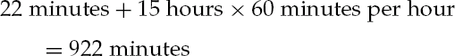
On October 6, 2003, the nearby and second expirations of the S&P 500 index options are the October 17,2003, and November 21, 2003, respectively, and the number of days to expiration are 12 and 47 days inclusive of the current date and the expiration date. The current date and expiration date are already incorporated, however. The number of minutes until midnight on the current date is 922, and the number of minutes from midnight on the day before expiration until time of expiration on the expiration day is 510. Thus, we reduce the number of days to expiration for the nearby and second nearby expirations to 10 and 45 and compute the number of minutes. With 1,440 minutes in each 24-hour day, the number of minutes for the second component of the nearby contract is
| 10 days × 1,440 minutes per day = 14,400 |
and the number of minutes for the second component of the second nearby contract is
| 45 days × 1,440 minutes per day = 64,800 |
The total numbers of minutes for the two contract expirations are therefore
| Nearby contract: 922 + 14,400 + 510 = 15,832 |
and
Second nearby contract: 922 + 64,800 + 510 = 66,232
The times to expiration in years are then computed as
| T1 = 15,832/525,600 = 0.0301217656 |
and
| T2 = 66,232/525,600 = 0.1260121766 |
where 525,600 in the number of minutes in a calendar year (that is, 1,440 minutes per day times 365 days).
Step 3: Compute the interest accumulation factor for each option expiration. The interest accumulation factor is defined as the terminal amount that $1 will accumulate to by the option's expiration if invested at the risk-free rate of interest. On October 6,2003, the risk-free rate corresponding to the nearby expiration was 0.920% on an annualized basis, and the risk-free rate corresponding to the second nearby expiration was 0.850% (On this particular day, the yield curve of the risk-free rate was inverted at short maturities.) The accumulation factors for the nearby and second nearby contracts were
and
respectively
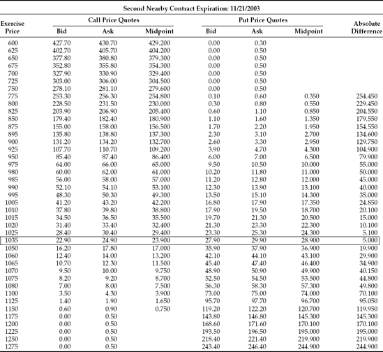
Step 4: Identify the at-the-money options for each option expiration. To identify the at-the money options for each expiration, we must first compute the bid/ask midpoints for all calls and puts with the nearby and second nearby contract expirations. This is shown in Tables 16.5 and 16.6. For each exercise price for which a call price and put price are available, compute the absolute difference between the call price and put price. Note that the calls and puts with zero bid prices are excluded for consideration. Such options appear in bold face. The exercise price with the lowest absolute difference is defined as the at-the-money option. On October 6,2003, the nearby at-the-money exercise price is 1030 (as is shown in Table 16.5 and the second nearby exercise price is 1035 (as is shown in Table 16.6).
Step 5: Compute the forward index level for each contract expiration. With the identity of the at-the-money options known, we compute the implied forward index level using the forward value version of put-call parity, that is,
For the nearby at-the-money options, the forward price is
F1 = 1030 + 1.0002771586449(13.500 —12.400) = 1031.10
For the second nearby at-the-money options, the forward price is
F2 = 1025 + 1.0010716773370(29.400 − 26.600) = 1029.99
Step 6: Identify the option series used in the computation of the VIX. In computing the VIX, only the prices of out-of-the-money calls and puts are used. To distinguish between in-the-money and out-of-the-money options, the exercise price just below the implied forward price (Xi,0) is used. The out-of-the-money calls are those with exercise prices greater than or equal Xi ,0, and the out-of-the-money puts are those with exercise prices less than or equal to Xi,0. If any of these option series have a bid price equal to zero, they are eliminated from consideration (In the event that the bid prices of two calls (puts) at adjacent exercise prices are equal to zero, all call (put) option series with higher (lower) exercise prices are eliminated even though they may nonzero bid pries). For the nearby and second nearby option series in the illustration, the exercise prices just below the forward index levels are X1,0 = 1030 and X2 0 = 1035. Since this procedure identifies two options (a call and a put) at exercise price Xi ,0, the arithmetic average of the call and put prices is used.
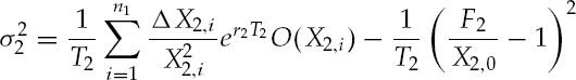
Step 7: Compute the implied variance for each contract expiration. The formula for computing the implied variance for the nearby contract is
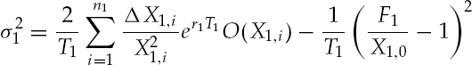
where T1 is the nearby contract month's time to expiration expressed in years, n1 is the number of out-of-the-money option series for the nearby contract month, X1, i is the exercise price of the ith option, r1 is the interest rate corresponding to option's expiration date, F1 is the forward index level implied by the at-the-money call and put prices, O(X1, i) is the bid/ask price midpoint of the nearby option with an exercise price of X1, and X1,0 is the exercise price just below the implied nearby forward price. The summation term also includes the at-the-money options. For the at-the-money options, the average of the call and put midpoints is used as O(X1,;). Finally, the term
Table 16.5. Nearby S&P 500 Index Option Prices Used in the Computation of the VIX on October 6, 2003, at 8:38 AM (CST)
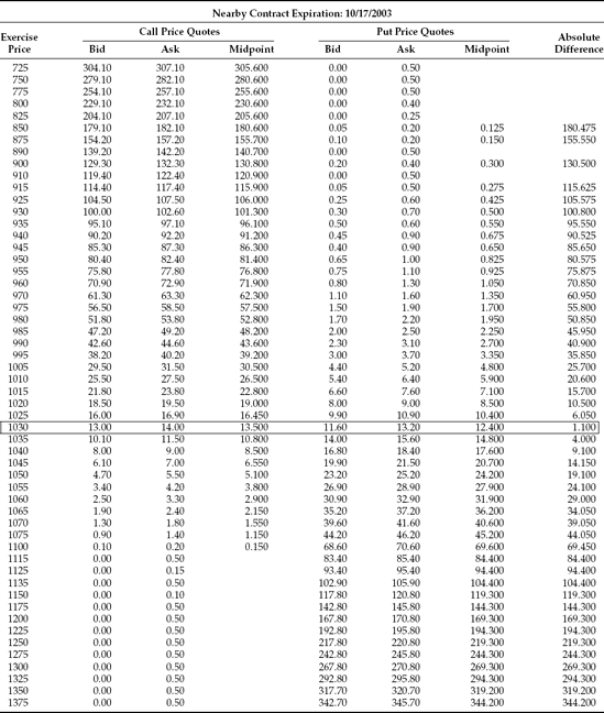 |
Table 16.6. Second Nearby S&P 500 Index Option Prices Used in the Computation of the VIX on 6, 2003, at 8:38 AM (CST)
|
The same procedure is used to compute the second nearby implied variance,
To illustrate the mechanics of these computations, first compute the values of the last term on the right-hand side (that is, the displacement factors) of the nearby and second nearby contracts. For the nearby contract,
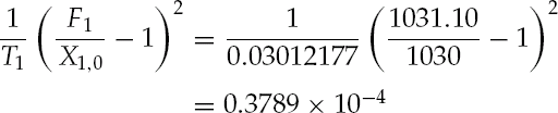
and, for the second nearby contract,
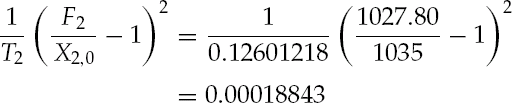
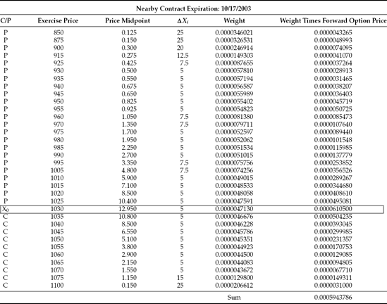
Next, take the sum in the first term on the right-hand side. Table 16.7 shows the values of each of the n1 terms for the nearby contract, and Table 16.8 shows the values of each of the n2 terms of the second nearby contract. The first term in the nearby contract's summation is
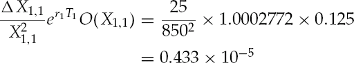
as is shown in Table 16.7. Note that the option price used in the expression is the forward price (that is, the current price carried forward until the end of the contract's life). The sum of the weighted average of the forward option prices is 0.0005943786 for the nearby contract and 0.0025376773 for the second nearby contract. The variance of the nearby contract is therefore
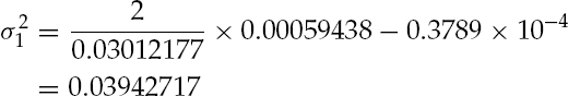
and the variance of the second nearby contract is
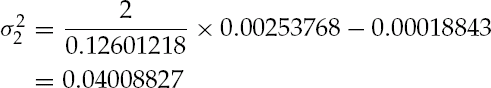
Table 16.7. Nearby S&P 500 Index Option Prices Computation to the composition of the VIX on October 6, 2003, at 8:38 AM (CST)
 |
Step 8: Compute the annualized volatility over the next 30 calendar days. The variances of the nearby and second nearby contracts correspond to times to expiration of T1 years and T2 years, respectively. VIX, however, maintains a constant time to expiration of 30 days or 30/365 = 0.0821917808 years. To find the variance over the 30 calendar-day interval, we must interpolate between the variances of the nearby and second nearby contracts, that is,
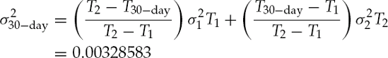
To compute the level of VIX, we annualize the 30-day variance and take the square root, that is,
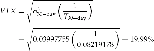
This is precisely the level of VIX reported by the CBOE at 8:38 AM (CST) on October 6.
Bollen, N.P.B., and Whaley, R. E. (2004). Does net buying pressure affect the shape of implied volatility functions? Journal of Finance 59, 2: 711–754.
Chicago Board Options Exchange (2003). VIX: CBOE volatility Index. Working paper.
Day, T.,E., and Lewis, C. M. (1992). Stock market volatility and the information content of stock index options. Journal of Econometrics 52: 267–287.
Demeterfi, K., Derman, E., Kamal, M., and Zou, J. (1999). More than you ever wanted to know about volatility swaps. Quantitative Strategies Research Notes, Goldman Sachs, working paper.
Dunbar, N. (2000). Inventing Money: The Story of Long-Term Capital Management and the Legends Behind It. Chichester, UK: John Wiley & Sons.
Fleming, J. (1998). The quality of market volatility forecasts implied by S&P 100 index option prices. Journal of Empirical Finance 5: 317–345.
Grossman, S. (1988). An analysis of the implications for stock and futures price volatility of program trading and dynamic hedging strategies. Journal of Business 61: 275–298.
Heston, S. L., and Nandi, S. (2000). Derivatives on volatility: Some simple solutions based on observables. Federal Reserve Bank of Atlanta working paper.
Lowenstein, R. C. (2000). When Genius Failed: The Rise and Fall of Long-Term Capital Management. New York: Random House.
Sulima, C. L. (2001). Volatility and variance swaps. Capital Market News Federal Reserve Bank of Chicago, March: 1–4.
Whaley, R. E. (1993). Derivatives on market volatility: Hedging tools long overdue. Journal of Derivatives 1: 71–84.
Whaley, R. E. (2000). The investor fear gauge. Journal of Portfolio Management 26, 3: 12–17.
Whaley, R. E. (2002). Return and risk of CBOE buy-write monthly index. Journal of Derivatives 10, 2: 35–42.
Whaley, R. E. (2006). Derivatives: Markets, Valuation, and Risk Management. Hoboken, NJ: John Wiley & Sons.