
ANTHONY F. L. PECORE
Research Analyst, Franklin Templeton Investments
Abstract: Life insurance is an asset and can be sold into a willing market. For years, life insurance companies served as the only market, paying cash surrender value. In recent years, the life-settlement market has developed to give competitive market pricing, rather than cash surrender value, to policyholders for their unneeded insurance. Development of a risk framework for life settlements requires an understanding of the mortality risk and expected cash flows.
Keywords: life settlement, life expectancy (LE), mortality risk
Life settlements are a new asset class for the investor. We believe life settlements possess investment characteristics that will be very attractive to those in search of investment-grade credit quality, long duration, assets priced at attractive spreads, with low correlation to other capital markets. The purpose of the chapter is to introduce the life settlement cash flow to asset managers, survey the driving valuation factors, and provide a first-order analytical framework for risk management.
After a policy owner has made the economic decision that their life insurance policy is no longer needed, they may seek to sell the policy or lapse the policy and accept the cash surrender value, if any, from the issuing insurance company. If the policy owner sells the policy to an investor, the investor will pay all future premiums and receive the policy's benefit upon the demise of the insured. Consider a policy with a $100 benefit, with premiums of $3 per year and a cash surrender value of $0. In this example, the investor would pay $25, $25 more than the insurance company would offer, for the policy and would have to pay the $3 per year premium to keep the policy in force. From the investor's perspective, both the acquisition cost and premiums are negative cash flows. If the insured matured 10 years after the sale, the investor would receive $100. This cash flow would have an internal rate of return (IRR) of roughly 7.5%. Of course, we don't know in advance how long the insured will live, but we can make assumptions based on actuarial and medical data. This cash flow uncertainty is not unusual for participants in the bond market. Many bond market investments contain cash flows where there is uncertainty in either the timing or value of a given cash flow. For example, mortgage-backed securities (MBSs) and credit default swaps (CDSs) possess these cash flow uncertainties, yet are large and mature markets.
In this section, we describe the investment characteristics of life settlement. They include:
Attractive IRRs and longer duration
Low correlation to other asset classes
High credit quality
The numbers used in the deterministic cash flow example were typical of those in the life settlement market place: policies are being purchased from individuals with life expectancies (LEs) typically greater than eight years. In its simplest form, there is no coupon payment in the life-settlement transaction; rather, there is capital appreciation supported by regular premium payments. The large benefit payment that is made at the insured's maturity provides for the life settlement's long duration. The discount at which policies can be purchased provides for the higher expected IRRs, which should compensate the investor for the asset's lack of liquidity and regulatory risk.
Life settlement cash flows consist of an outflow of premium payments followed by a benefit inflow. In the simplest form, both the premium payments and the benefit are known quantities. What is not specifically known are the timing of the benefit payout and the duration of premium payments. The timing of the cash flows is dependent on the remaining life span of the insured. Thus, the ultimate return of the life settlement is not correlated to economic cycles, but rather to the life expectancy of the insured.
The fundamental credit risk to the investor in life settlements is that the issuing life insurance company fails to pay the benefit. Three points help to protect the investor:
Through guaranty funds many states protect up to $300,000 in benefits if a carrier is in default when policy claim is filed.
Insurance claims sit at the top of an insurance company's capital structure, and must be paid before any form of loan.
Life settlements can be selected from only investment-grade companies.
Purchasing policies from lower-rated insurers is possible, and the investor may be rewarded for assuming the higher risk.
The fair market value of a life-settlement policy is the expected net present value of the policy face, less the expected net present value of the premiums required to keep the policy in force. The probabilities required to calculate expectations on a single life of both policy face and premium cash flows will be developed and described in actuarial terms. With the probability of a cash flow occurring tied to the life status of the underlying insured, both expectations and variances of cash flows can be calculated. We show how the value of a policy increases in time. A portfolio of policies will then be considered and expressions developed to quantify risk in terms familiar to financial management. Throughout, we will be concerned with the question of how much cash flow to expect in any given year given today's information.
While today's actuarial theory incorporates the many insights of, and could be entirely cast in the framework of, modern probability theory, a working knowledge of actuarial math can be built from the life-table concept. The earliest actuarial studies for life insurance and annuity purposes began with the development of the life table. The following overview of actuarial methods is primarily drawn from Gerber (1997) and Chiang (1983).
In a life table, a cohort of a suitably large population was established, and at the end of the year, the remaining number of survivors was marked. (Sir Edmund Halley, of comet fame, is credited with constructing the first life table in 1693.) A life table following a cohort of 10,000 initially 75-year-old females with the same initial health and demographic conditions is given in Table 59.1. The table is truncated at year 100. Column t marks the beginning of the interval year. Column Age, x is the age of remaining survivors at time t. Column lx is the number of survivors at time t. Column dx is the number of people who survived to age x, then passed within the following year.
The quantities d and l are integer values counting the number of survivors and matured. The quantities p and q are ratios or probabilities of survival or death and range between 0 and 1. Before deriving the remaining columns, note that of the initial 10,000 individuals, only 697 survive to age 100, and that half of the original cohort has passed by approximately 13.5 years.
Table 59.1. Life Table of 10,000 Initially 75-Year-Old Females
t | Age, x | lx | dx | qx | px | t p75 | t p75 q75+t |
|---|---|---|---|---|---|---|---|
Note: Table derived from the ultimate table for 75-year-old females drawn from the Female Non-Smoking 2001 Valuation Basic Table (commonly referred to as the VBT2001 tables). | |||||||
0 | 75 | 10000 | 238 | 0.02375 | 0.97625 | 1.00000 | 0.02375 |
1 | 76 | 9763 | 255 | 0.02610 | 0.97390 | 0.97625 | 0.02548 |
2 | 77 | 9508 | 273 | 0.02869 | 0.97131 | 0.95077 | 0.02728 |
3 | 78 | 9235 | 291 | 0.03155 | 0.96845 | 0.92349 | 0.02914 |
4 | 79 | 8944 | 310 | 0.03464 | 0.96536 | 0.89436 | 0.03098 |
5 | 80 | 8634 | 329 | 0.03808 | 0.96192 | 0.86338 | 0.03288 |
6 | 81 | 8305 | 356 | 0.04285 | 0.95715 | 0.83050 | 0.03559 |
7 | 82 | 7949 | 383 | 0.04824 | 0.95176 | 0.79491 | 0.03835 |
8 | 83 | 7566 | 405 | 0.05357 | 0.94643 | 0.75656 | 0.04053 |
9 | 84 | 7160 | 426 | 0.05945 | 0.94055 | 0.71604 | 0.04257 |
10 | 85 | 6735 | 445 | 0.06609 | 0.93391 | 0.67347 | 0.04451 |
11 | 86 | 6290 | 453 | 0.07200 | 0.92800 | 0.62896 | 0.04528 |
12 | 87 | 5837 | 474 | 0.08113 | 0.91887 | 0.58367 | 0.04735 |
13 | 88 | 5363 | 486 | 0.09064 | 0.90936 | 0.53632 | 0.04861 |
14 | 89 | 4877 | 491 | 0.10076 | 0.89924 | 0.48771 | 0.04914 |
15 | 90 | 4386 | 482 | 0.10994 | 0.89006 | 0.43857 | 0.04822 |
16 | 91 | 3904 | 445 | 0.11402 | 0.88598 | 0.39035 | 0.04451 |
17 | 92 | 3458 | 425 | 0.12283 | 0.87717 | 0.34584 | 0.04248 |
18 | 93 | 3034 | 413 | 0.13628 | 0.86372 | 0.30336 | 0.04134 |
19 | 94 | 2620 | 402 | 0.15346 | 0.84654 | 0.26202 | 0.04021 |
20 | 95 | 2218 | 388 | 0.17488 | 0.82512 | 0.22181 | 0.03879 |
21 | 96 | 1830 | 357 | 0.19508 | 0.80492 | 0.18302 | 0.03570 |
22 | 97 | 1473 | 318 | 0.21588 | 0.78412 | 0.14732 | 0.03180 |
23 | 98 | 1155 | 252 | 0.21788 | 0.78212 | 0.11551 | 0.02517 |
24 | 99 | 903 | 206 | 0.22837 | 0.77163 | 0.09035 | 0.02063 |
25 | 100 | 697 | 171 | 0.24585 | 0.75415 | 0.06971 | 0.01714 |
The number of lives in the cohort aged x is lx. The number of lives at the end of t years later is lx+t. The ratio of those initially aged surviving t years and is the expected
The number of maturities through t years is lx — lx+t The ratio of maturities through t years to the initial number of lives is x
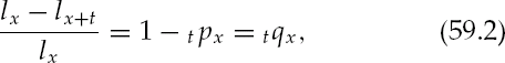
and can be expressed in terms of the percentage of survivors.
When the time span t is limited to 1 year the pre-subscript t is dropped. The notation px is read "the percentage of lives aged x, surviving one year is px." The notation qx is read "the percentage of lives aged x, maturing within one year is qx." Defining the number of maturities within one year as dx = lx — lx+1 the percentage of those initially aged x maturing within one year can also be written
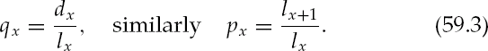
The relation px + qx = 1 is immediate. The probability of an individual aged x being alive or dead within one year is 100%. The probability qx is the quantity given in actuarial tables.
The probability of an individual initially aged x living for t years then maturing in the interval (t, t + 1) is the conditional probability
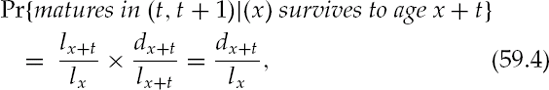
or using the actuarial notation,
Note that
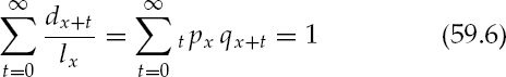
which expresses the sum of all maturities is equal to the original number of lives in the cohort, or the probability of maturing in some year in the future is 100%.
The probability of an individual initially aged x living for t years can also be expressed as the product
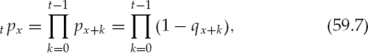
and is read as the probability of an individual aged x living to x + 1 and then living from x + 1 to x + 2 and so on. Equation (59.7) is particularly useful given that only qx are provided in actuarial tables.
Referring to Table 59.1, the number of survivors at the beginning of year t = 3 is l78 = 9235, these survivors are all 78-years-old. At the end of year 3, t = 4, l79 = 8944. Accordingly, 310 individuals, who began the year at age 78 passed before their 79th birthday and d78 = 310. The percentage of 78-year-olds who passed compared to those who entered the year alive is q78 = 3.155%, and with a sufficiently large population q78 is the probability that a 78-year-old non-smoking female will pass before her 79th birthday.
The probability that a 75-year-old non-smoking female will live to 78, then pass before her 79th birthday can be calculated with either (59.4) or (59.5).
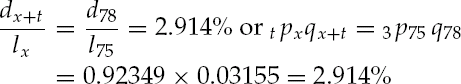
Both methods give the same result, but qx is again typically given in actuarial tables, and working directly with them is preferred.
The life expectancy of an individual aged x is
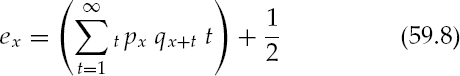
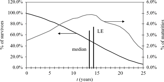
The 1/2 represents the fraction of the final year of life that lived. The life expectancy for the cohort in Table 59.1 is 13.64 years. In this case, the life expectancy is approximately one year longer than the median life, or point in time at which only 1/2 of the cohort survives.
Figure 59.1 shows how the cohort is expected to evolve over time. The survivor curve begins with 100% of the cohort alive and declines as individuals mature. The time at which 50% of the cohort has matured is the median remaining life. The LE is slightly longer than the median remaining life.
The life table is a binomial process. A 78-year-old female has a 1 — q78 chance of living to her 79th birthday and a q78 of not. The variance for the estimates in any given year x is
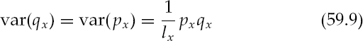
The variance of the survivor estimate t years from today is
The variance in the estimate of those expected to survive t years, then pass within the next year, is
In each case, lx is the number of independent trials, or in the context of the life table, the number of individuals in the individual cohort.
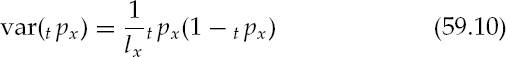
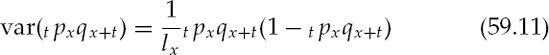
First, consider the whole life contract, which provides a payment or death benefit of one unit at the end of the year of death. Using the preceding cohort described in Table 59.1, what is the net present value (NPV) of the whole life policy benefit? Using a discount factor of v, where r is the discount rate,
a maturity in year T, received at time t = T + 1 has the NPV of vT+1. While the amount payment is known, the time of payment, T, is random. Define Z as a random variable
The expected NPV of Z is the probability-weighted cash flow of benefits is
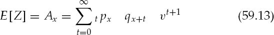
The term Ax is known as the net single premium where a payment of Ax would purchase a paid up whole-life policy requiring no further premiums.
The NPV of a term policy's benefits follows from (59.13) where benefits after year n are zero, resulting in a truncated series:
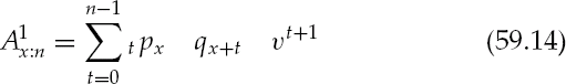
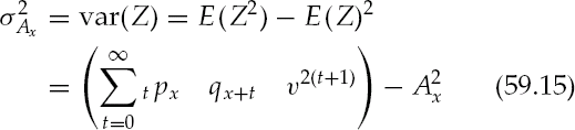
The variance of Z is
A whole-life annuity-due pays one unit as long as the beneficiary is alive. Payments are issued at the beginning of each year the contract is in force at time t = 0,1, 2, 3 ... The NPV of this cash flow is
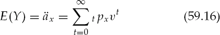
Paying one unit rather than receiving while the insured is alive would match the cash flow of a level premium.
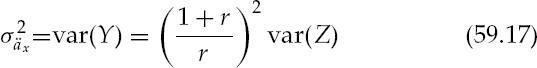
The variance is of the whole-life annuity is
Values for the quantities Ax and äx, one period forward can be quickly seen from a binomial tree construction:
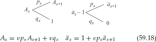
Today's value Ax can be understood as the discounted value of the one period forward value Ax+1 assuming survival plus the discounted benefit value assuming maturity. Today's value äx is the discounted value of the one period forward äx+1 plus an immediate payment of one unit.
The annual level premium Π required to keep a whole life policy with benefit F in force is found by using (59.13) and (59.16).
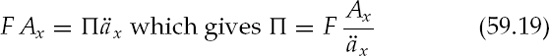
With the proper level premium, the NPV of the whole life benefit should be equal to the NPV a whole life annuity. Dividing the premium Π by the benefit F results in the premium to face ratio (pfr) or πx
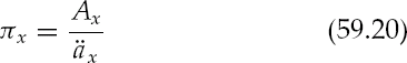
This premium is unloaded; it does not include expense loadings, which include acquisition costs, collection expenses, administration fees, or risk loadings for larger benefits. Typical values for π in life settlement market range from 3% to 7%.
The unloaded minimum cost of insurance for a one-year term paid, in the event of death, at the end of the term with a premium paid in advance is expressed as a pfr and is simply qx.
The analysis developed so far has assumed a base case survivor curve and reflects the survival rates for a large population sharing major factors such as age, gender, and smoking status. The life table allows the calculation of qx, which is expressed either as the ratio of maturities in a given year to those alive at the beginning of the year, or the probability that a living individual will mature within one year.
An individual health status will likely vary from the average of its cohort. If an individual is very ill, compared to their cohort, they may have four times the chance of maturing within a year. However, a healthy individual with evidence of superior cardiovascular health may have 0.9 times the chance of maturing within a year when compared to their base cohort. Some individuals may experience higher mortality risk while exposed to the hazard of some ailment such as cancer, but return to standard health once cured.
The mortality risk relative to the cohort base is expressed with the multiplier mk which can vary with time. The Multiple Medical Impairment Study gives mortality multipliers, based on experience from 1962 to 1977 for various impairment groups. Though the study is dated it provides a framework and example baseline from which to consider multiple medical impairments.
Depending on the medical impairment, the multiplier can decay in time. One reason is that an individual may be diagnosed with a condition, which, if survived the first few years, would return to the base risk. A second reason would be that as a person ages with impaired health, their cohort is likely to experience the same impairment. An example of the former is an individual who experiences higher mortality risk while exposed to the hazard such as cancer, but returns to standard health once cured. Cardiovascular disease is an example of the later.
Equations (59.5) and (59.7) are combined to give and expression for the probability of maturity in a given year with multiplier m:
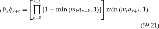
The min() function ensures that the quantity mtqx+t never exceeds 1, as the probability of maturity in a given year can never exceed 100%.
Figure 59.2 shows the mortality distributions 70 years with notable health risk, and an 80-year-old with minor health concerns. For simplicity, the multipliers are constant 350% and 130%, respectively. The distributions are nearly equivalent in shape as are the median and life expectancy. Note that the life expectancy for the 70-year-old is more sensitive to a change in multiplier m than the life expectancy of the 80-year-old.
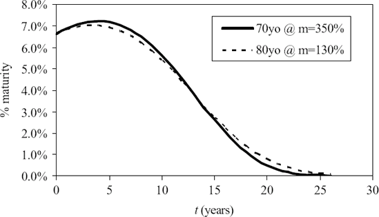
Figure 59.2. Mortality Distributions for a 70-Year Old with Notable Health Impairment and an 80-Year Old with Minor Health Concerns
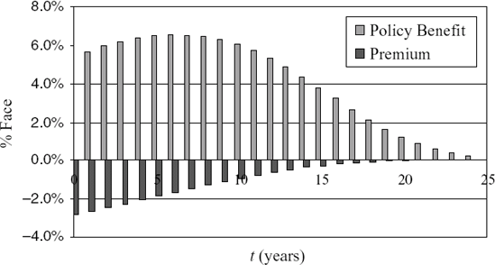
Figure 59.3. Illustrative Cash Flows for Cohort Of 80-Year Old Nonsmoking Females with Level Premiums Of 3% of Face
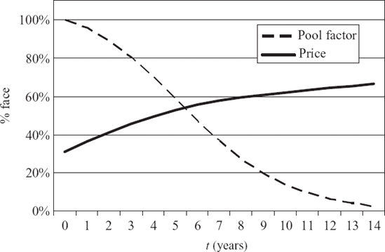
Insurance industry underwriting convention adjusts for substandard health by underwriting a policy at a table rating of 0,1,2,3... The table rating tr, relates to the multiplier m by
While the table rating at issue can often be found stated within the policy, the underlying actuarial tables that are used in the policy construction are not public knowledge.
The net present value (NPV) of the policy benefit less the NPV of the premium stream is the value of the life settlement. Using the actuarial quantities Ax and äx developed (59.13) and (59.16), where the effect of substandard mortality is expressed through the multiplier m, the value of the life settlement is

where P is the policy value or price and F is the policy face, Φ is the premium to face ratio. The discount rate or IRR of the life settlement is embedded in the quantities Ax (m) and äx (m). The policy value expressed as a percentage of face is p. Illustrative cash flows are shown in Figure 59.3. The NPV of these cash flows gives the policy value.
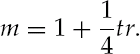
Equation (59.19) assumes a level premium and level policy face, and no loan against the policy, but can be easily generalized to account for such variations. Using the expression for forward values in (59.18), we can project the forward values of the life settlement. Figure 59.4 shows how the price of the policy is expected to increase at future dates.
The expected net present value of the policy face less the expected NPV of the premiums required to keep the policy in force has been established in (59.22). We will now combine Npolicies together into a portfolio. Price and other attributes are averaged together using policy face weighting. Assuming each individual life in the portfolio is uncorrelated, a variance estimate for the portfolio price is given. Having paid a known price, this variance can be used to estimate the more useful quantity the variance of the expected IRR do to actuarial variance.
In dollar terms, the value of the ith policy in a portfolio of life settlements is
Summing all policies
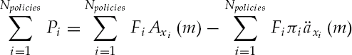
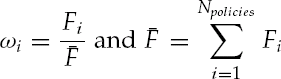
Dividing by the total face amount in the portfolio gives the face weighted value Φ
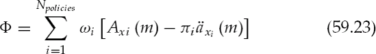
where
The variance of the portfolio price is
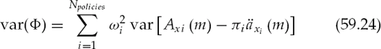
where
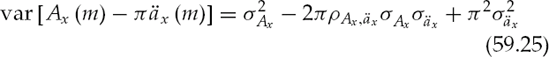
and σAx and σäx are defined in (59.15) and (59.17) and ρAx,äx = -l;
Table 59.2. Calculated Variance Using Monte Carlo (MC) Simulation
Npolicies | 1 | 5 | 10 | 50 | 100 |
|---|---|---|---|---|---|
MC:σ2Ax | 0.051440 | 0.010299 | 0.005164 | 0.001027 | 0.000514 |
MC:σ2äx | 4.481010 | 0.897156 | 0.449853 | 0.089423 | 0.044782 |
MC:σ2Φ | 0.090537 | 0.018127 | 0.009089 | 0.001807 | 0.000905 |
Table 59.3. Analytical Variance for Various Number of Policies
Npolicies | 1 | 5 | 10 | 50 | 100 |
|---|---|---|---|---|---|
Eq. (59.15): σ2Ax | 0.051466 | 0.010293 | 0.005147 | 0.001029 | 0.000515 |
Eq. (59.17): σ2äx | 4.483290 | 0.896658 | 0.448329 | 0.089666 | 0.044833 |
Eq. (59.26): σ2Φ | 0.090583 | 0.018117 | 0.009058 | 0.001812 | 0.000906 |
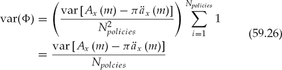
Now consider a portfolio with N independent lives from the same cohort, where each policy has the same face. The face weighting for each policy is ωi = 1/Npolicies, and because each life is from the same cohort, the variance is also the same for each policy. The variance of the portfolio is
To confirm the analytical expressions for variance in (59.15), (59.17), and (59.26), we calculate the variance of a portfolio of Npolicies using Monte Carlo simulation (see Table 59.2) and compare to the analytical values.
Comparing Table 59.2 to Table 59.3 shows agreement between calculated and analytical value. As demonstrated, calculating
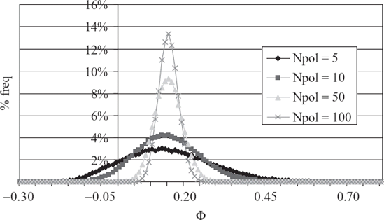
Table 59.4. Comparison of Standard Deviation in r Using Monte Carlo (MC) Simulation and Analytical Approximation
Npolicies | 5 | 10 | 50 | 100 | 300 | 500 |
|---|---|---|---|---|---|---|
MC:σr | 0.17879 | 0.09353 | 0.03063 | 0.02026 | 0.01168 | 0.00889 |
Eq. (59.27): σr | 0.08748 | 0.06186 | 0.02766 | 0.01956 | 0.01129 | 0.00875 |
err | - 51.1% | - 33.9% | - 9.7% | - 3.5% | - 3.3% | - 1.6% |
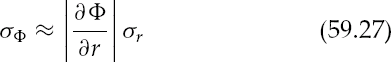
Assuming a portfolio of policies was assembled using a discount rate of r¯ for a price-to face-ratio of Φ, what is the expected variance of r? We can connect the standard deviation of Φ, σΦ with σr via
with
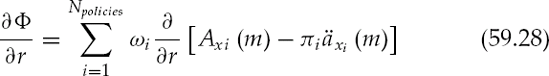
where
The standard deviation σr can be approximated directly from actuarial information and (59.27)-(59.29). To confirm this result, we calculate the standard deviation of r, σr, for a portfolio of Npolicies from the same cohort priced at Φ using Monte Carlo simulation and compare to the analytical approximation.
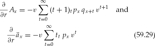
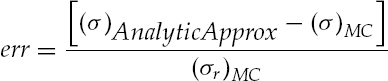
The results in Table 59.4 show converging agreement between the two measures of σr with increasing Npolicies. The error measure between the Monte Carlo results and the analytical is
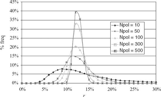
The resulting distributions from the Monte Carlo distribution in r are shown in Figure 59.6. As expected, the distribution tends toward the normal distribution as the number of policies increase.
A life settlement is the sale of a life insurance policy, while the insured is still alive, from the policy's original owner to a potentially unrelated third party. If the policy were allowed to lapse, the owner would be essentially selling the policy for cash surrender value. In recent years, the life-settlement market has developed to give competitive market pricing, which may exceed a policy's cash surrender value, to policyholders for their unneeded insurance.
The lifespan of the insured, which is arguably uncor-related to other assets, is the primary factor driving the life settlement cash flow. The life expectancy of the underlying insured is typically greater than eight years which accounts for the life settlement's long duration. Because policies sit atop of the capital structure of high credit quality insurance carriers, the risk of credit default is minimal.
Standard actuarial methods to develop a valuation methodology for single policies and a portfolio of policies can be employed. We show how the valuation methodology can be used to calculate forward price values of the portfolio. Assuming a binomial process, an estimate for the variance of the portfolio's expected internal rate of return is given and compared to Monte Carlo simulations.
Black, K. Jr., and Skipper, H. D. Jr., (2000). Life and Health Insurance. Upper Saddle River, NJ: Pearson Education.
Booth, P. M., Chadburn, R., Cooper, D., Haberman, S., and James, D. (1998), Modern Actuarial Theory and Practice. Boca Raton, FL: Chapman & Hall/CRC.
Chiang, C. L. (1983). Life Table and Its Applications, Malabar, FL: Krieger Publishing Co.
Daykin, C. D., Pentikainen, T., and Pesonen, M. (1993). Practical Risk Theory for Actuaries Boca Raton, FL: Chapman & Hall/CRC.
Deshpande, J. V., Purohit, S. G. (2005). Life Time Data: Statistical Models and Methods. Singapore: World Scientific Publishing Co.
Gerber, H. U. (1997). Life Insurance Mathematics, 3rd edition. New York: Springer-Verlag.
Klugman, S. A., Panjer, H. H., and Willmot, G. E. (1998). Loss Models: From Data to Decisions. New York: Wiley-Interscience.
Luenberger, D. G (1998). Investment Science. New York: Oxford University Press.
Multiple Medical Impairment Study (1998). Staff MIB, SOA AAIM HOLUA-IHOU Mortality & Morbidity Liaison Committee, Center for Medico-Actuarial Statistics of MIB Inc.