Creating and Laying Out a PivotTable

You can create a PivotTable either from a database table or from a range of data. If you have a database table already, as in the example, you can create the PivotTable from that. Otherwise, create the database table you'll use, or enter the data in a worksheet as usual without creating a database table.

Once your data is ready, you can create a PivotTable either automatically or manually. Which works best depends on your data and what you're trying to do with it, but often you can save time by creating a PivotTable automatically and then adjusting it as necessary. If an automatic PivotTable turns out not to be what you need, you can create the PivotTable manually from scratch instead.

Creating a PivotTable Automatically

To create a PivotTable automatically, follow these steps:

1. Open the workbook and display the worksheet that contains the table or data you'll use in the PivotTable.
2. Click in the table that you'll use for the PivotTable. If you'll use a range rather than a named table, select the range.
3. Choose Data Analysis PivotTable from the Ribbon, clicking the main part of the PivotTable button. You can also click the PivotTable pop-up button, then click Create Automatic PivotTable on the pop-up menu, but there's no advantage to doing so. Excel then does the following:
   • Inserts an automatic PivotTable on a new worksheet
   • Gives the new worksheet a default name such as Sheet5
   • Displays the PivotTable Builder window
   • Adds the PivotTable tab to the Ribbon and displays it
   • Displays some information about PivotTables the first time you create one

Figure 12–2 shows the automatic PivotTable produced from the sample data table, with the PivotTable Builder window positioned in front of the worksheet.

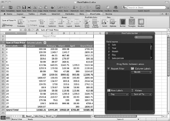
Figure 12–2. The quickest way to create a PivotTable is to have Excel create it automatically. You will usually need to adjust the PivotTable using the PivotTable Builder window to make the PivotTable show the information you want. Depending on the data you're using, the PivotTable may look substantially different from this one.

After creating a PivotTable automatically, you'll normally need to adjust it. This is because Excel seldom guesses exactly which information you need where.

To adjust a PivotTable, use the techniques you'll learn in the next section, which shows you how to build a PivotTable from scratch.

Creating a PivotTable Manually

If creating an automatic PivotTable doesn't give a useful result or if you prefer to do things by hand, you can build the PivotTable manually using the PivotTable Builder.

To create a PivotTable manually, follow these steps:

1. Open the workbook, and display the worksheet that contains the table or data you'll use in the PivotTable.
2. Click in the table that you'll use for the PivotTable. If you'll use a range rather than a named table, select the range.
3. Choose Data Analysis PivotTable Create Manual PivotTable from the Ribbon or Data PivotTable from the menu bar to display the Create PivotTable dialog box (see Figure 12–3). If you're using a named table, you can also choose Tables Tools Summarize with PivotTable from the Ribbon; if you're using a range, this command isn't available.
   

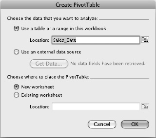
   Figure 12–3. In the Create PivotTable dialog box, choose the table or range of data from which to create the PivotTable. Then choose between putting the PivotTable on a new worksheet or an existing worksheet.

4. In the Choose the data that you want to analyze area at the top of the Create PivotTable dialog box, select the Use a table or a range in this workbook option button.

   NOTE: Instead of creating a PivotTable from data in a worksheet, you can create a PivotTable from an external data source such as a FileMaker database or Access database. To do so, you select the Use an external data source option button in the Choose the data that you want to analyze area of the Create PivotTable dialog box, click the Get Data button, then choose the data source. Before you can do this, you must install an Open Database Connectivity (ODBC) driver to enable Excel to connect to the data source, as discussed in Chapter 10.

5. Make sure the Location text box shows the table or range you want to use. If you clicked in the table or selected the range in step 2, you'll be all set. If not, type in the table name or click and drag in the worksheet to select the range (click the Collapse Dialog button first to get the Create PivotTable dialog box out of the way first if necessary).
6. In the Choose where to place the PivotTable area of the Create PivotTable dialog box, choose the appropriate option button:
   • New worksheet. Select this option button if you want to place the PivotTable on a new worksheet. This is often clearest, because it gives you plenty of room for the PivotTable.
   • Existing worksheet. Select this option button if you want to place the PivotTable on an existing worksheet. Click in the Location text box, click the worksheet's tab, then click and drag in the worksheet to enter the location.
7. Click the OK button to close the Create PivotTable dialog box. Excel positions a PivotTable framework on a new worksheet or the existing worksheet you chose and displays the PivotTable Builder window. Figure 12–4 shows the PivotTable framework on a new worksheet named Sheet4.

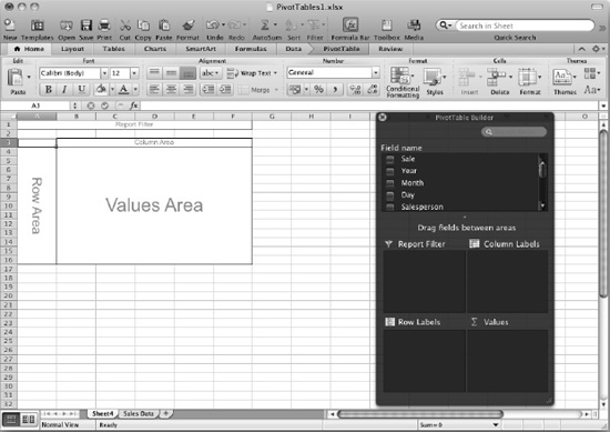
Figure 12–4. When you insert a PivotTable manually, Excel creates an empty framework on which you lay out the PivotTable the way you need it.

Now that you've inserted the framework for the PivotTable, you can add fields to it from the Field name list box in the PivotTable Builder window.

Understanding How the PivotTable Framework and PivotTable Builder Window Work

Take a moment to look at the PivotTable framework and the PivotTable Builder window. You use the PivotTable Builder window to arrange the fields on the PivotTable framework.

Here are the essentials you need to know:

• Field name list box. This list box in the PivotTable Builder window contains an entry for each of the fields that Excel found in the data table or range you chose. Each item in the list has a check box that you can select to add the field to the PivotTable. The PivotTable framework has no matching area for the Field name list box, because the fields go into the various areas of the PivotTable when you use them.

• Report Filter. This area at the top of the PivotTable acts as a filter for the PivotTable as a whole, narrowing down the rest of the table to only the data that matches your filter. For example, if you put the Salespeople field in the Report Filter area by dragging it to the Report Filter box in the PivotTable Builder window, you get a pop-up menu of your salespeople from which you choose whose data you want to show. As you'll see later in this chapter, you can filter by one field, two fields, or more.
• Row Area. This area at the left of the PivotTable shows the row headings. You designate those headings by dragging the appropriate field or fields to the Row Labels box in the PivotTable Builder window.
• Column Area. This area at the top of the PivotTable shows the column headings. You choose those headings by dragging the appropriate field or fields to the Column Labels box in the PivotTable Builder window.
• Values Area. This area in the body of the PivotTable—in most cases the main part of the PivotTable—contains the values. You specify the values by dragging the appropriate field or fields to the Values box in the PivotTable Builder window.

If this is hard to grasp, don't worry. You'll see how PivotTables work in just a moment.

Adding the Fields to the PivotTable Framework

To create the PivotTable, you add fields to the PivotTable framework by dragging fields to the Report Filter box, the Row Labels box, the Column Labels box, and the Values box in the PivotTable Builder window.

Which fields you need to drag where depends on your data source and what you're trying to make it show. Here's a walk-through using the fields in the data source. If you're using the sample data source, your results should look similar; if your data source is different, they'll look different, but the PivotTable will work in much the same way.

In the Field name list box in the PivotTable Builder window, click the Year field and drag it to the Report Filter box. Excel selects the Year check box, enters Year in cell A1, and creates a pop-up menu for selecting the years in cell B1 (see Figure 12–5).

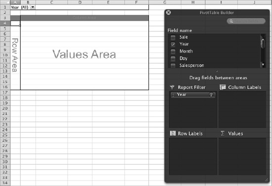
Figure 12–5. Drag the Year button from the Field name box in the PivotTable Builder window to the Report Filter box to create the Year pop-up menu shown in cell B1 here. Excel selects the (All) item in the pop-up menu at first, making the PivotTable show all the years.

1. In the Field Name list box, click the Salesperson field and drag it to the Row Labels box. Excel selects the Salesperson check box and creates a row label for each salesperson's name (see Figure 12–6).
   

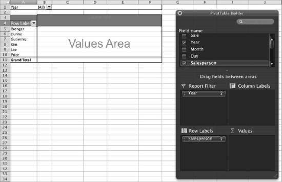
   Figure 12–6. Moving the Salesperson button to the Row Labels box makes Excel create a row label from each salesperson's name.

2. Drag the Line field from the Field name list box in the PivotTable Builder window to the Column Labels box. Excel selects the Line check box in the Field name list box and adds the product lines as column labels (see Figure 12–7).
   

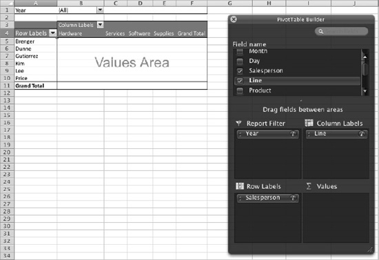
   Figure 12–7. Drag the Line item from the Field name list box in the PivotTable Builder window to the Column Labels area. Excel adds the product lines as column labels and selects the Line check box for you.

3. Now click the Total Price field in the Field name list box, and drag it to the Values box in the PivotTable Builder window. Excel adds to the PivotTable the values of the items the salespeople sold (see Figure 12–8).

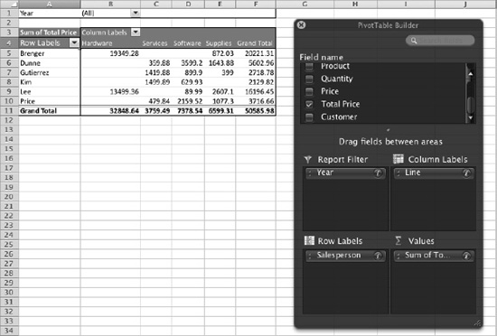
Figure 12–8. Drag the Total Price field from the Field name list box to the Values box in the PivotTable Builder window to add the totals of each salesperson's sales to the PivotTable.

This gives us a PivotTable that shows how much of each product line each salesperson sold. At first, the PivotTable shows (All) in the Year pop-up menu in the Report Filter area. To see a breakdown by a year, open the Year pop-up menu,then click the year you want.

This is useful—but it's just the start of what you can do with the PivotTable.

Changing the PivotTable to Show Different Data

The great thing about PivotTables is how easy they are to change to show different data. You can change a PivotTable by adding different fields to it, removing fields it's currently using, or rearranging the fields among the Report Filter box, the Column Labels box, the Row Labels box, and the Values box in the PivotTable Builder window.

Here are four examples of how you can change the basic PivotTable created earlier in this chapter. These examples work as a sequence, so you'll need to make each change in turn if you want to work through them.

• In the Field name list box, click the Product field,then drag it to the Row Labels box in the PivotTable Builder window. Excel adds a list of the product names of the products each salesperson has sold (see Figure 12–9).

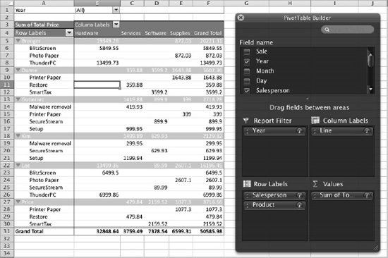
Figure 12–9. Drag the Product field to the Row Labels box in the PivotTable Builder window to add a list of the products each salesperson has sold. You can collapse any list by clicking the disclosure triangle to the left of the salesperson's name.

• In the Row Labels box in the PivotTable Builder window, drag the Salesperson field below the Product field. The PivotTable then shows each product with a collapsible list of the salespeople who have been selling it (see Figure 12–10).

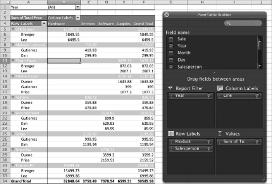
Figure 12–10. Drag the Salesperson field below the Product field in the Row Labels box in the PivotTable Builder window to produce a list of products showing the salespeople who have been selling them.

• Drag the Product field from the Row Labels box in the PivotTable Builder window to the Column Labels box. Then drag the Line field from the Column Labels box outside the PivotTable Builder window and drop it, making it disappear from the PivotTable. (You can also clear the Line check box in the Field name list box.) These changes produce a PivotTable showing the salespeople by row and what they've sold of the products in columns (see Figure 12–11).
  

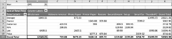
  Figure 12–11. Removing the product lines and making column labels of the products produces this PivotTable that shows how much each salesperson has sold of each product.

• Make the following changes to see which of your product lines each of your customers bought in a specific period:

1. Drag the Month field from the Field name list box in the PivotTable Builder window to the Report Filter box, placing it below the Year field. You can now filter by month as well as by field. For example, you can choose 2011 as the Year filter, then choose January as the Month filter to see only your January 2011 results.
2. In the Field name list box, clear the Salesperson check box to remove the Salesperson field from the Row Labels area. Then drag the Customer field from the Field name list box to the Row Labels box instead, making the PivotTable show one customer in each row.
3. In the Field name list box, clear the Product check box to remove the Product field from the Column Labels area. Then drag the Line field to the Column Labels box to make the PivotTable show the product lines in the columns. Figure 12–12 shows the resulting PivotTable.

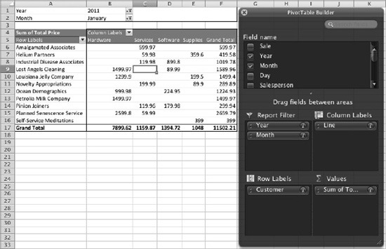
Figure 12–12. You can add the Month field to the Report Filter box, putting it below the Year field, to filter your PivotTable by first the year (here, 2011) and then the month (here, January). This PivotTable shows how much customers bought from each product line in January 2011.

When you've finished working with the PivotTable Builder window, you can close it by clicking the Close (x) button at the left end of its title bar or by choosing PivotTable View Builder from the Ribbon.

If you need to open the PivotTable Builder window again, choose PivotTable View Builder from the Ribbon.

Changing the Function Used to Summarize a Field

When you add values to a PivotTable, Excel tries to automatically use the right function for the calculation that type of data needs. For example, when you add a field that shows prices, Excel uses the SUM() function on the assumption that you want to add the values. And if you use nonnumeric data such as names, Excel uses the COUNT() function, giving you the number of different items.

If you need to change a field to a different function, follow these steps:

Click the field, or click a cell containing data that the field produces.

1. Choose PivotTable Field Settings from the Ribbon to display the PivotTable Field dialog box (see Figure 12–13).
   

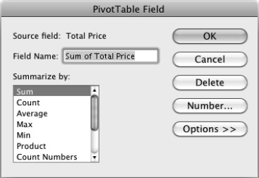
   Figure 12–13. In the PivotTable Field dialog box, you can change the formula used to summarize the field's data.

2. In the Summarize by list box, click the function you want to use. For example, click the Average function if you want the field to show an average instead of a sum. Excel automatically changes the contents of the Field Name text box to reflect the function you chose—for example, changing the text from Sum of Total Price to Average of Total Price.

   TIP: If you need to present the data in a different format (for example, as the amount of difference from a base value), click the Options button in the PivotTable Field dialog box to expand the dialog box and reveal more options. In the Show data as pop-up menu, choose the format you want—for example, Difference From. Then select the base field in the Base field list box and the base item in the Base item list box.

3. If you want to change the field name, type the change in the Field Name text box.
4. Click the OK button to close the PivotTable Field dialog box.