Identifying Unusual Values with Conditional Formatting

In many worksheets, it's useful to be able to monitor the values in the cells and to pick out values that stand out in particular ways. For example, you may want to see which ten products are bringing in the most revenue, or you may need an easy way to make unusually high values or unusually low values stand out from the others.

To monitor the values in a cell or a range, you can apply conditional formatting—formatting that Excel displays only when the condition is met. For example, if you're monitoring temperatures in Fahrenheit, you could apply conditional formatting to highlight low temperatures (say, below 20F) and high temperatures (say, above 100F). Temperatures in the normal range would not receive any conditional formatting, so the low temperatures and high temperatures would jump out on the worksheet.

Understanding Excel's Preset Types of Conditional Formatting

Excel provides five kinds of preset conditional formatting, which you can apply from the Conditional Formatting panel in the Format group of the Home tab of the Ribbon. Figure 4–15 shows the Conditional Formatting panel with the Icon Sets panel displayed.

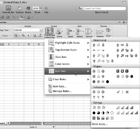
Figure 4–15. The Conditional Formatting panel includes sets of icons you can apply to indicate data trends.

• Highlight Cells Rules. This panel gives you an easy way to set up conditional formatting using Greater Than, Less That, Between, Equal To, Text that Contains, A Date Occurring, or Duplicate Values criteria.
• Top/Bottom Rules. This panel lets you apply conditional formatting for Top 10 Items, Top 10 %, Bottom 10 Items, Bottom 10 %, Above Average, and Below Average criteria.
• Data Bars. This panel enables you to apply different gradient fills and solid fills.
• Color Scales. This panel lets you set up color scales using two or three colors—for example, using green, amber, and red to indicate different levels of risk associated with activities.
• Icon Sets. This panel provides different sets of icons, such as directional arrows (up, sideways, down) or a checkmark–exclamation point–cross set, for indicating data trends.

Applying a Preset Form of Conditional Formatting

To apply one of the preset forms of conditional formatting, open the Conditional Formatting panel, display the appropriate panel from it, click the type of formatting, and then specify the details. For example:

1. Select the cell or range you want to affect.
2. Choose Home Format Conditional Formatting Highlight Cells Rules Greater Than to display the New Formatting Rule dialog box (see Figure 4–16).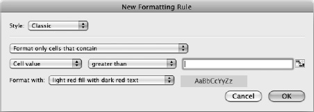
   

   Figure 4–16. Excel's preset conditional formatting types make it easy to apply conditional formatting to cells quickly.

3. In the Style pop-up menu, you can choose a different style for the conditional formatting if you want. Excel automatically selects the style that suits the type of conditional formatting you chose—in the example, Classic.
4. The Comparison pop-up menu below the Style pop-up menu shows the comparison for the type of conditional formatting—in the example, Format only cells that contain. You can choose a different comparison if necessary, but you won't normally need to do so.
5. On the next line of controls, set up the comparison. In the example, the first pop-up menu is set to Cell value, and the second pop-up menu is set to “greater than” because this is a Greater Than rule. In the third box, you enter the comparison. You can either type in the value or collapse the dialog box, click the cell that contains the value, and then restore the dialog box.
6. In the Format with pop-up menu, choose the formatting you want. Excel provides various canned options, but you can also create custom formatting by clicking the custom format item at the bottom of the list and working in the Format Cells dialog box that opens. (This is a cut-down version of the Format Cells dialog box you met earlier in the chapter—it has only the Font tab, the Border tab, and the Fill tab.)
7. Click the OK button to close the New Formatting Rule dialog box. Excel applies the conditional formatting.

Creating Custom Conditional Formatting

If none of the preset conditional formatting rules meets your needs, you can define conditional formatting rules of your own. To do so, follow these steps:

1. Select the cell or range you want to affect.
2. Choose Home Format Conditional Formatting New Rule to display the New Formatting Rule dialog box.
3. In the Style pop-up menu, choose the type of conditional formatting: 2-Color Scale, 3-Color Scale, Data Bars, Icon Sets, or Classic. The New Formatting Rule dialog box display controls for creating that type of conditional formatting. Figure 4–17 shows the New Formatting Rule dialog box with the controls for creating an icon set displayed.
   

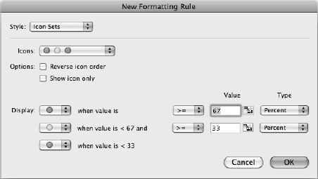
   Figure 4–17. When none of the conditional formatting rules is what you need, use the New Formatting Rule dialog box to create a custom rule.

4. Use the controls to specify what conditional formatting the rule will apply. For example, for the Icon Sets style shown in Figure 4–17, you could do the following:
   • Open the Icons pop-up menu, and then click the set of icons you want to use as the basis for the formatting.
   • In the Options area, select the Reverse icon order check box if you want to use the icon sequence the other way around—for example, green-yellow-red instead of red-yellow-green. Select the Show icon only check box if you want the icon to appear without the value that produced it; this can be good for simplifying complex worksheets, but it may prompt too many questions about values to be worth using.
   • In the Display area, open each pop-up menu, and choose the symbol to use (or simply accept the default symbol). Then use the controls to set up the condition, value, and type.
5. When you've finished creating the rule, click the OK button to close the New Formatting Rule dialog box.

Changing the Order in Which Excel Applies Conditional Formatting Rules

Many cells and ranges need only one type of conditional formatting applied—but others may need two or more types. When you apply multiple types of conditional formatting, you may need to change the order Excel applies the conditional formatting rules in. Or you may simply need an easy way to see which conditional formatting rules you've applied to a particular cell or range.

To see which conditional formatting rules you've applied to cells, and to change the order, follow these steps:

1. Select the cell or range you're interested in.
2. Choose Home Format Conditional Formatting Manage Rules to display the Manage Rules dialog box (see Figure 4–18).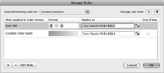
   

   Figure 4–18. Use the Manage Rules dialog box to check which conditional formatting rules you've applied to a cell or range and to change the order Excel uses the rules.

3. Verify that the Show formatting rules for pop-up menu shows Current Selection rather than another range. If not, choose Current Selection.
4. In the list box in the center of the Manage Rules dialog box, look through the list of rules. Change the rules or their order as needed.
   • Change the order of the rules. Click the rule you want to move, go to the Change rule order area, and then click the Move Up button (the up arrow) or the Move Down button (the down arrow), as needed.
   • Delete a rule. Click the rule, and then click the Remove (–) button.
   • Edit a rule. Click the rule, click the Edit Rule button, and then work in the Edit Formatting Rule dialog box. This dialog box has the same controls as the New Formatting Rule dialog box.
   • Create a new rule. Click the Add (+) button, and then work in the New Formatting Rule dialog box, as discussed in the previous section. When you finish creating the rule, move it up the list to where it belongs.
   • Apply the rule to a different range. In the rule's Applies to column, click the Collapse Dialog button to collapse the Manage Rules dialog box. Select the appropriate range, and then click the Collapse Dialog button again to restore the Manage Rules dialog box.
   • Stop evaluating other rules if a rule is true. Select the rule's check box in the Stop if true column.
   • Click the OK button to close the Manage Rules dialog box. Excel applies your choices to your selection.

Clearing Conditional Formatting from a Cell, Range, or Worksheet

If a cell, range, worksheet, table, or PivotTable no longer needs conditional formatting, clear it as follows:

1. Choose the item:
   • Select the cell or range.
   • Click in the table or PivotTable.
   • Activate the worksheet.
2. Choose Home Format Conditional Formatting Clear Rules, and then click the appropriate item on the submenu: Clear Rules from Selected Cells, Clear Rules from Entire Sheet, Clear Rules from This Table, or Clear Rules from This PivotTable.