
Troubleshooting Common Problems with Formulas
Formulas are great when they work, but a single-letter typo or a wrong reference can prevent a formula from working correctly. This section shows you how to deal with common problems with formulas, starting with solutions to the error messages you're most likely to produce.
CAUTION: This section shows you how to troubleshoot problems that Excel can identify because they prevent your calculations from working. But what can be much more dangerous are mistakes in formulas that don't cause errors but instead give the wrong results; because the formulas work correctly, Excel can't detect the errors and so raises no objections, but the values you get aren't what you intend. If having your calculations give the correct results is important to you (as is usually the case), have a competent colleague check your worksheets for mistakes. You may also want to get a book such as Spreadsheet Check and Control (O'Beirne, Systems Publishing), which teaches you how to audit Excel worksheets.
Understanding Common Errors—and Resolving Them
Excel includes an impressive arsenal of error messages, but some of them appear far more frequently than others. Table 5–3 shows you eight errors you're likely to encounter, explains what they mean, and tells you how to solve them.
Table 5–3. How to Solve Excel's Eight Most Common Errors
| Error | What the Problem Is | How to Solve It |
| ##### | The formula result is too wide to fit in the cell. | Make the column wider—for example, double-click the column head's right border to AutoFit the column width. |
| #NAME? | A function name is misspelled, or the formula refers to a range that doesn't exist. | Check the spelling of all functions; correct any mistakes. If the formula uses a named range, check that the name is right and that you haven't deleted the range. |
| #NUM! | The function tries to use a value that is not valid for it—for example, returning the square root of a negative number. | Give the function a suitable value. |
| #VALUE! | The function uses an invalid argument—for example, using =FACT() to return the factorial of text rather than a number. | Give the function the right type of data. |
| #N/A | The function does not have a valid value available. | Make sure the function's arguments provide values of the right type. |
| #DIV/0 | The function is trying to divide by zero (which is mathematically impossible). | Change the divisor value from zero. Often, you'll find that the function is using a blank cell (which has a zero value) as the argument for the divisor; in this case, enter a value in the cell. |
| #REF! | The formula uses a cell reference or a range reference that's not valid—for example, because you've deleted a worksheet. | Edit the formula and provide a valid reference. |
| #NULL! | There is no intersection between the two ranges specified. | Change the ranges to produce an intersection. |
CAUTION: The =SUM() function is smart enough to ignore text values that you feed it. For example, if cell A1 contains the value 1 and cell A2 contains the text Dog, the function =SUM(A1:A2) returns 1 even though the formula =A1+A2 returns a #VALUE! error. The =SUM() function's smartness here is a mixed blessing: you get a usable result, which is presumably what you want—but this hides the mistake you've made in trying to add text instead of a numerical value.
Seeing the Details of an Error in a Formula
When Excel identifies an error in a formula, it displays a green triangle at the upper-left corner of the cell that contains the formula. Click the cell to display an action button that you can hold the mouse over to display a ScreenTip explaining the problem (as shown on the left in Figure 5–6) or click to display a menu of actions you can take to resolve the problem (as shown on the right in Figure 5–6).
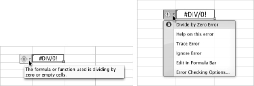
Figure 5–6. Hold the mouse pointer over the action button for an error cell to display a ScreenTip explaining what's wrong.
Tracing an Error Back to Its Source
To see which cell is causing an error, click the error cell, then choose Formulas ![]()
Audit Formulas ![]()
Check for Errors ![]()
Trace Error. Excel displays an arrow from the cell or cells causing the error to the error cell. The left screen in Figure 5–7 shows a simple example of tracing an error; the more complex the worksheet, the more helpful this feature is. Excel displays a worksheet symbol (see the right screen in Figure 5–7) if the cell reference is on another worksheet or in another workbook.
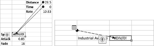
Figure 5–7. Use the Formulas ![]() Audit Formulas
Audit Formulas ![]() Check for Errors
Check for Errors ![]() Trace Error command to identify the cell or cells causing an error. If the cell reference is on another worksheet or in another workbook, Excel displays a worksheet symbol, as shown on the right.
Trace Error command to identify the cell or cells causing an error. If the cell reference is on another worksheet or in another workbook, Excel displays a worksheet symbol, as shown on the right.
NOTE: If you've turned off background error checking in the Error Checking preferences pane, choose Formulas ![]()
Audit Formulas ![]()
Check for Errors (clicking the main part of the Check for Errors button) from the Ribbon or Tools ![]()
Error Checking from the menu bar to check for errors.
Displaying All the Formulas in a Worksheet
When you need to review or check all the formulas in a worksheet, choose Formulas ![]()
Function ![]()
Show ![]()
Show Formulas, placing a check mark next to the Show Formulas item on the Show pop-up menu. Excel displays the formulas and automatically widens the worksheet columns to give you more space (see Figure 5–8).
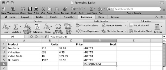
Figure 5–8. Choose Formulas ![]()
Function ![]()
Show ![]()
Show Formulas when you need to see all the formulas in a worksheet.
When you've finished viewing the formulas, choose Formulas ![]()
Function ![]()
Show ![]()
Show Formulas again, removing the check mark from the Show Formulas menu item. Excel automatically restores the columns to their former widths.
Seeing Which Cells a Formula Uses
To see which cells a formula uses, or to trace errors, click the cell that contains the formula, and then choose Formulas ![]()
Audit Formulas ![]()
Trace Precedents. Excel displays an arrow showing the formula back to its roots. If one of the cells the formula uses contains a formula itself, you can click that cell and click the Trace Precedents button again to display its precedents in turn. Figure 5–9 shows the precedents of cell D6 and one of the cells that it uses, cell D2.
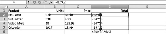
Figure 5–9. Use the Trace Precedents command to see which cells you're using to produce a formula result. In this example, cells B2 and C2 go to make up the formula in cell D2, which in turn appears in the =SUM(D2:D5) formula in cell D6.
When you need to look at the problem the other way and see which formulas use a particular cell, click the cell, and then choose Formulas ![]()
Audit Formulas ![]()
Trace Dependents. Again, Excel displays arrows, this time from the cell going to each of the formulas that use it. Figure 5–10 shows an example of tracing dependent cells.
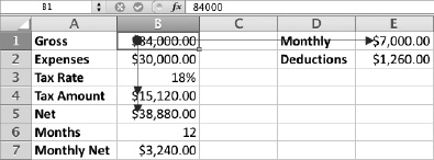
Figure 5–10. Use the Trace Dependents command to see which formulas use a particular cell's value to produce their results.
NOTE: You can use the Trace Precedents command and the Trace Dependents command either with formulas displayed or with formula results displayed, whichever you find most useful.
When you've finished tracing precedents and dependents (or errors), choose Formulas ![]()
Audit Formulas ![]()
Remove Arrows (clicking the main part of the Remove Arrows button) to remove the arrows from the screen. If you want to remove just precedent arrows or dependent arrows, click the Remove Arrows pop-up button, and then click the Remove Precedent Arrows item or the Remove Dependent Arrows item on the pop-up menu.
Removing Circular References
Even if you're careful, it's easy enough to create a circular reference—one that refers to itself.
Circular references most often occur when you enter a formula that refers to a cell that itself refers to the cell in which you're entering the formula. For example, say cell A1 contains the formula =B1. If you enter the formula =A1 in cell B1, you've created a circular reference: cell B1 gets its value from cell A1, which gets its value from cell B1, and so on.
You can also enter a circular reference by making a cell refer to itself. For example, if you enter =A1/B1 in cell A1, you've created a circular reference in that cell, because cell A1 refers to itself. This type of circular reference is usually easier to avoid than the previous type.
Circular references can be useful in some specialized circumstances, such as when you need to perform iterations of a calculation, but normally you don't want them in your worksheets, so Excel helps you to get rid of them.
When you create a circular reference that Excel can't calculate, Excel displays the Excel Cannot Calculate a Formula dialog box shown in Figure 5–11. Click the OK button if you want to open a Help window showing information on how to deal with circular references, or click the Cancel button if you want to go ahead and enter the circular reference in the cell (for example, because you can tell what the problem is and will be able to fix it easily).
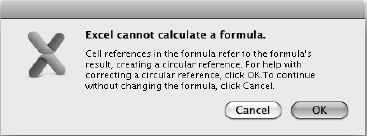
Figure 5–11. Circular references can cause problems in worksheets, so Excel warns you when you enter one. You can click the Cancel button if you're sure you want to create the circular reference.
NOTE: If you leave circular references in a worksheet, use the Circular readout on the status bar to identify them. This readout shows the location of the most recent circular reference that Excel has identified. When you've dealt with that circular reference, the Circular readout shows the next one, and so on, until there are none left.