Examining Different Scenarios in a Worksheet

Often, when you've built a worksheet, you'll want to experiment with different data in it. For example, if you're setting budgets, you may need to play around with different figures for the different departments to get the overall balance you require.

You can experiment with different data by changing the values directly in your worksheet—but then you may need to restore your original values afterward. Another approach is to create multiple copies of the worksheet (or of the workbook) and then change the values in the copies, leaving the original untouched. This works fine, but if you then need to change the original worksheet (for example, adding another column of data), the changes quickly become messy.

Instead of working in these awkward ways, you can use Excel's scenarios. A scenario is a way of entering different values into a set of cells without changing the underlying values. You can switch from one scenario to another as needed, and you can merge scenarios from different versions of the same worksheet into a single worksheet.

Creating the Worksheet for Your Scenarios

Start by creating the workbook and worksheet you'll use for your scenarios. If you have an existing workbook with the data in it, open it up. Set up the data and formulas in your worksheet as usual.

Figure 11–7 shows the sample worksheet this section uses as an example. The worksheet summarizes the financial returns from a modest portfolio of rental properties.

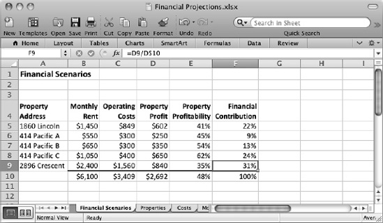
Figure 11–7. To start using scenarios, create a worksheet containing your existing data and the formulas needed.

Here's what you see on the worksheet:

• The Property Address column shows each property's address.
• The Monthly Rent column shows each property's monthly rent. Cell B10 contains a SUM() formula to produce the total rent. Each of the cells here has a name to make it easy to recognize—Rent_Lincoln, Rent_Pacific_A, and so on.
• The Operating Costs column shows the monthly operating cost for each property, including all mortgage costs and other financial horrors. Cell C10 uses a SUM() formula to produce the total running cost. The numbers in this column are rounded. Each of these cells has a name: Costs_Lincoln, Costs_Pacific_A, and so on. Again, this is so that we can refer to the cells easily and clearly.
• The Property Profit column shows how much profit each rental unit returns after subtracting the operating cost from the rent (for example, cell D5 contains the sum =B5-C5). The numbers in this column are rounded; that's why cell D5 appears to contain a math error but is in fact correct. Cell D10 uses a SUM() formula to return the total profit.
• The Property Profitability column shows the property's profitability as a percentage. To produce the profitability figure, we divide the Property Profit value by the Monthly Rent value—for example, cell E5 contains the formula = D5/B5. At the bottom of the column, cell E10 uses an AVERAGE() formula to show the average profitability of the properties.
• The Financial Contribution column shows each property's contribution to the total profit as a percentage. To produce the contribution figure, we divide each property's profit by the total profit in cell D10. For example, cell F9 contains the formula =D9/D$10, using a mixed reference to keep the row absolute when copying the formula. Cell F10 contains a SUM() formula that adds the percentages, letting us see that they total 100%.

Times are bad, and the total profit is too low. So, we'll use scenarios to see how we can improve matters by raising rents and shaving costs.

Opening the Scenario Manager Dialog Box

When you're ready to start working with scenarios, choose Data Analysis What-If Scenario Manager from the Ribbon or Tools Scenarios from the menu bar to display the Scenario Manager dialog box. At first, when the workbook contains no scenarios, the Scenario Manager dialog box appears as shown in Figure 11–8.

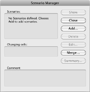
Figure 11–8. At first, the Scenario Manager dialog box contains nothing but a prompt telling you to click the Add button. Do so.

Creating Scenarios

After opening the Scenario Manager dialog box, you can create your scenarios.

To create a scenario, follow these steps:

1. From the Scenario Manager dialog box, click the Add button to display the Add Scenario dialog box (see Figure 11–9).
   

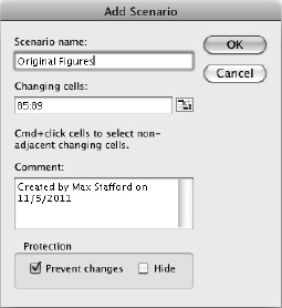
   Figure 11–9. Use the Add Scenario dialog box to set up each scenario. First create a scenario for your original data so that you can easily return to it.

2. In the Scenario name text box, type a descriptive name for the scenario.
3. Click in the Changing Cells text box, and then enter the details of the cells that users of the scenario are allowed to change. For the original scenario, we're not making changes; but for a scenario that involves changing the rent, the range is cells B5:B9.
   • Click and drag in the worksheet to select a range of contiguous cells. If you need to select noncontiguous cells, click the first one, and then Cmd+click each other cell.

   NOTE: When you enter a cell or a range of cells in the Changing Cells text box by clicking in the worksheet, Excel changes the name of the dialog box from Add Scenario to Edit Scenario. Odd though this seems, it's normal.

   • You can also type the name of a range into the Changing cells text box.
   • There's a Collapse Dialog button to the right of the Changing Cells text box, but you don't need to use it, because Excel automatically collapses the Add Scenario dialog box when you click in the worksheet. After you've selected the changing cells, Excel expands the dialog box again.
4. In the Comment text box, type a comment that explains what the scenario is and how to use it. Excel creates a default comment of Created by, your user name (as set in the Office applications), and the date, but a descriptive comment is usually more helpful.
5. Choose settings as needed in the Protection area at the bottom of the dialog box:
   • Prevent changes. Select this check box when you need to prevent changes to the scenario. To make the protection take effect, you'll need to protect the worksheet as described in the next section.
   • Hide. Select this check box when you need to prevent others from seeing this scenario—for example, because you want them to experiment with their own figures rather than looking at yours. Again, you need to protect the worksheet.
6. Click the OK button to close the Add Scenario dialog box or Edit Scenario dialog box. Excel displays the Scenario Values dialog box (see Figure 11–10). This dialog box shows a text box for each of the changing cells in the scenario. Here's where you see the benefit of naming the changing cells—each text box is easy to identify. If you haven't named the changing cells, the cell addresses appear, and you may need to refer to the worksheet to see which cell is which.
   

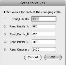
   Figure 11–10. In the Scenario Values dialog box, enter the values to use for the new scenario you're creating. The cell names produce the labels (Rent_Lincoln and so on), which are much easier to refer to than cell addresses (for example, B5).

7. Change the values as needed for the scenario.

   TIP: You can type formulas into the text boxes in the Scenario Values dialog box. For example, to increase the Rent_Lincoln value in Figure 11–10 by 25 percent, you could change the 1450 value to the formula =1.25*1450. After you enter formulas like this, Excel displays the dialog box shown in Figure 11–11 when you close the Scenario Values dialog box, telling you that it has converted names and results of formulas to values. Click the OK button.

   

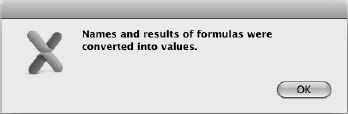
   Figure 11–11. After you enter formulas in the Scenario Values dialog box, Excel automatically converts them to values for you.

8. Click the OK button to close the Scenario Values dialog box. Excel returns you to the Scenario Manager dialog box, where the scenario now appears in the Scenarios list box.

To add another scenario, click the Add button in the Scenario Manager dialog box, and then repeat the previousprocess.

Applying Protection to Your Scenarios

If you selected either the Prevent Changes check box or the Hide check box in the Protection area of the Add Scenario dialog box or the Edit Scenario dialog box, you need to protect the worksheet to make the protection take effect.

To protect the worksheet, follow these steps:

1. If the Scenario Manager dialog box is open, click the Close button to close it.
2. Choose Tools Protection Sheet from the Ribbon or Tools Protection Protect Sheet from the menu bar to display the Protect the sheet and contents of locked cells dialog box.
3. Type a password in the Password text box and again in the Verify text box.
4. In the Allow users of this sheet to box, make sure the Edit Scenarios check box is cleared.
5. Click the OK button to close the dialog box. Excel applies the protection.
6. Save the workbook. For example, press Cmd+S or click the Save button on the Standard toolbar.

After protecting the scenarios in the worksheet like this, you'll need to turn off the protection before you can edit the scenarios. To turn off the protection, choose Tools Protection Sheet from the Ribbon or Tools Protection Unprotect Sheet from the menu bar, type the password in the dialog box that Excel displays, and then click the OK button.

Editing and Deleting Scenarios

From the Scenario Manager dialog box, you can quickly edit a scenario by clicking it in the Scenarios list box, clicking the Edit button, and then working in the Edit Scenario dialog box. Excel automatically updates the scenario's comment for you with details of the modification (for example, “Modified by Jack Cunningham on 02/18/2011”), but you'll often want to type in more details, such as what you're trying to make the scenario show.

When you no longer need a scenario, delete it by clicking the scenario in the Scenarios list box and clicking the Delete button. Excel doesn't confirm the deletion; but if you delete a scenario by mistake, and recovering it is more important than losing any other changes you've made since you last saved the workbook, you can recover the scenario by closing the workbook without saving changes (assuming the scenario was already saved in the workbook).

Switching Among Your Scenarios

Once you've created multiple scenarios for the same worksheet, you can switch among them by clicking the scenario you want in the Scenarios list box in the Scenario Manager dialog box (see Figure 11–12) and then clicking the Show button. Excel displays the scenario's figures in the worksheet's cells. The Scenario Manager dialog box stays open, so you can quickly switch to another scenario.

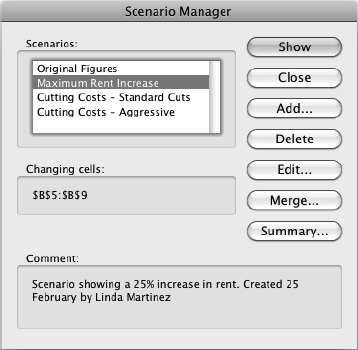
Figure 11–12. To switch to another scenario, click the scenario in the Scenarios list box in the Scenario Manager dialog box, and then click the Show button.

Merging Scenarios into a Single Worksheet

If you develop and share your scenarios in a single workbook, you can keep them all together. But sometimes you may need to develop your scenarios in separate workbooks and then combine them. You can do this easily by using the Merge command in the Scenario Manager dialog box.

To merge scenarios, follow these steps:

1. Open all the workbooks containing the scenarios you will merge.
2. Make active the workbook and worksheet you will merge the scenarios into.
3. Choose Data Analysis What-If Scenario Manager from the Ribbon or Tools Scenarios from the menu bar to display the Scenario Manager dialog box.
4. Click the Merge button to display the Merge Scenarios dialog box (see Figure 11–13).
   

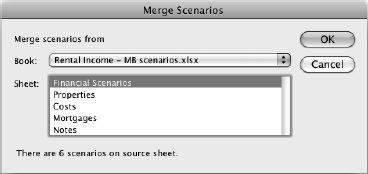
   Figure 11–13. In the Merge Scenarios dialog box, choose the workbook and worksheet that contain the scenarios you want to merge into the active workbook.

5. Open the Book pop-up menu, and choose the open workbook that contains the scenarios you want to merge in. The Sheet list box shows a list of the worksheets in the workbook.
6. In the Sheet list box, click the worksheet that contains the scenarios. The readout at the bottom of the Merge Scenarios dialog box shows how many scenarios the worksheet contains, which helps you pick the right worksheet.
7. Click the OK button. Excel closes the Merge Scenarios dialog box, merges the scenarios, and then displays the Scenario Manager dialog box again.

Creating Reports from Your Scenarios

Sometimes you can make the decisions you need by simply creating scenarios and looking at them in the worksheet. At other times, it's helpful to create a report from the scenarios so that you can compare them. Excel gives you an easy way to create either a summary report or a PivotTable report straight from the Scenario Manager dialog box.

To create a report from your scenarios, follow these steps:

1. Choose Data Analysis What-If Scenario Manager from the Ribbon or Tools Scenarios from the menu bar to display the Scenario Manager dialog box.
2. Click the Summary button to display the Scenario Summary dialog box (see Figure 11–14).
   

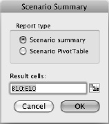
   Figure 11–14. In the Scenario Summary dialog box, choose between a scenario summary and a scenario PivotTable, and then select the result cells for the summary.

3. In the Report type box, select the Scenario summary option button if you want to create a summary worksheet. If you want to create a scenario PivotTable, select the Scenario PivotTable option button.
4. Click in the Result cells text box, and then enter the addresses of the cells whose results you want the report or PivotTable to show. You can type in addresses or range names or select the appropriate cells in the worksheet.
5. Click the OK button to close the Scenario Summary dialog box. Excel creates the report or PivotTable. Figure 11–15 shows a sample of a summary report, which Excel places on a new worksheet named Scenario Summary at the beginning of the workbook.

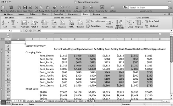
Figure 11–15. Excel places a summary report on a new worksheet named Scenario Summary at the beginning of the workbook.