Representing Data Graphically with Icon Sets

Another helpful way of representing data graphically is by using icon sets to indicate the relationship of a set of values to each other. For example, you can apply a set of directional arrows to make Excel show green up arrows on high values, yellow right-pointing arrows on midpoint values, and red down arrows on low values. Figure 8–10 shows this kind of icon set used to track the month-by-month and full-quarter performance of the five salespeople you met earlier in this chapter.

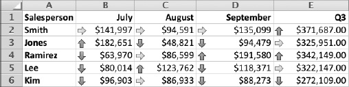
Figure 8–10. Apply an icon set to a range of cells to provide a quick visual reference to their relationship. This worksheet uses four icon sets—one on column B, one on column C, one on column D, and one on column E—rather than a single icon set, which would compare all the values in B2:E6 to each other and show that the third-quarter totals in column E made the monthly values look pretty miserable.

To apply an icon set to cells, follow these steps:

1. Enter the data that will produce the icon set.
2. Select the cells that contain the data.
3. Choose Home Format Conditional Formatting Icon Sets to display the Icon Sets panel (see Figure 8–11).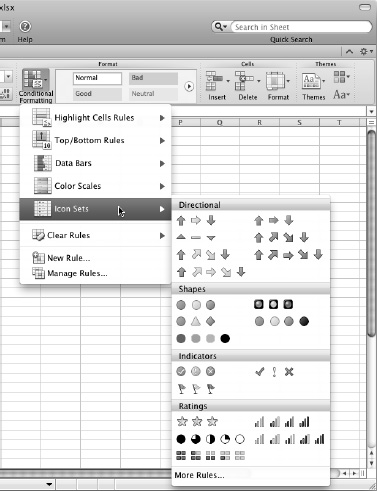
   

   Figure 8–11. On the Icon Sets panel, click the set of icons you want to apply to the selected cells.

4. Click the icon set you want to apply.

Many icon sets work straight out of the box (as it were), but you may need to adjust others as follows:

1. With the cells still selected, choose Home Format Conditional Formatting Manage Rules to display the Manage Rules dialog box (shown in Figure 8–4, earlier in this chapter).
2. Make sure the right rule is selected. If you've applied only one conditional formatting rule to the cells, it will be; if you've applied multiple rules, you may need to click the right rule.
3. Click the Edit Rule button to display the Edit Formatting Rule dialog box (see Figure 8–12).
   

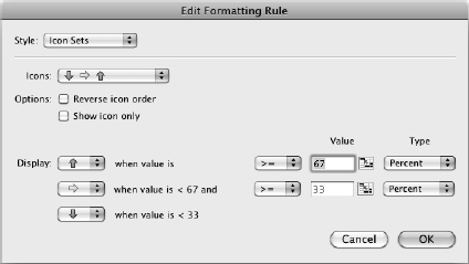
   Figure 8–12. In the Edit Formatting Rule dialog box, you can change the icons, reverse the order, show only the icons, and change the threshold values.

4. To change the icons used, open the Icons pop-up menu, then click the icon set you want.
5. If you want to show the icons in reverse order, select the Reverse icon order check box.
6. If you want to show the icons without the values that produce them, select the show icon only check box.

   TIP: When you want to show each value in one cell and its icon in another cell, set up the icon cells with formulas that refer to the value cells. For example, enter =B2 in cell C2, then apply an icon set to the icon cells, open the Edit Formatting Rule dialog box, and select the Show icon only check box.

7. In the Display area, choose the icons you want to use and the threshold values for them.
8. Click the OK button to close the Edit Formatting Rule dialog box. Excel returns you to the Manage Rules dialog box.
9. Click the OK button to close the Manage Rules dialog box and return to your worksheet, which shows the changes you made.