Creating Databases in Excel

When you need to store a lot of the same type of information in a worksheet, you can create a database in a table. For example, if you run a business, you can make a database of your customers and their orders.

The first step is to set up the table and to tell Excel that you're creating a table rather than a regular worksheet. The next step is to add your data to the table, either by typing it into the cells as usual or by using a data-entry form.

Once the data is in the table, you can sort the table to reveal different aspects of its contents or filter it to identify items that match the criteria you specify.

Understanding What You Can and Can't Do with Excel Tables

Before you start creating a table in Excel, it's important to be clear about what you can and can't do with Excel tables.

As you know, an Excel worksheet consists of rows and columns. To create a table on a worksheet, you make each row into a record—an item that holds all the details of a single entry. For example, in a table that records your sales to customers, a record would contain the details of a purchase. You make each column a field in the table—a column for the purchase number, a column for the date, a column for the customer's last name, and so on. Figure 10–1 shows part of an Excel table for tracking sales to customers.

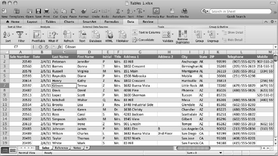
Figure 10–1. An Excel database consists of a table, with each row forming a record and each column containing a field.

This is what's called a flat-file database: all the data in the database is stored in a single table rather than in separate tables that are linked to each other.

This means you can use Excel to create any database for which you can store all the data for a record in a single row. Because you have a million rows at your disposal, you can create large databases if necessary, but they may make Excel run slowly.

What you can't do with Excel is create relational databases—ones that store the data in linked tables. A relational database is the kind of database you create with full-bore database applications such as FileMaker, Microsoft Access (on Windows), Oracle (on various operating systems), or SQL Server (on Windows). In a relational database, every record has a unique ID number or field that the application uses to link the data in the different tables.

Creating a Table and Entering Data

In this section, you'll look at how to create a table and enter data in it either by using standard Excel methods or by using a data-entry form.

Creating a Table

To create a table, follow these steps:

1. Create a workbook as usual. For example, you can:
   
   • Create a new blank workbook. Press Cmd+N or choose FileNew Workbook from the menu bar.
   • Create a workbook based on a template or an existing workbook. Press Cmd+Shift+P or choose FileNew from Template, then make your choices in the Excel Workbook Gallery dialog box.
2. Name the worksheet on which you'll create the table. Double-click the worksheet tab, type the name you want (up to 31 characters, including spaces), then press Return to apply the name.
3. Type the headings for the table. For example, if the table will contain customer names and addresses, you'd type fields such as Last Name, First Name, Middle Initial, Title, Address 1, and so on. Try to get all the fields in place at this point; you can add columns to the table later, but you'll then need to add extra data to the existing records.

   NOTE: Usually, it's easiest to put the headings in the first row of the worksheet, but if you need to have information appear above the table, leave rows free for it.

4. Format the headings differently from the rows below them. For example, click the row header for the heading row, then press Cmd+B to apply boldface.
5. Select the headings and at least one row below them.
6. Choose Tables Table Options New from the Ribbon, clicking the main part of the New button rather than the pop-up button. Excel makes the following changes:
   
   • Creates the table.
   • Gives the table a default name, such as Table1 or Table2.
   • Turns the header row into headers with pop-up buttons.

     NOTE: If your headings have the same formatting as the data rows, choose Tables Table Options New Insert Table with Headers rather than Tables Table Options New. Otherwise, Excel inserts a new row containing headers above your heading row. If your table doesn't have headers, choose Tables Table Options New Insert Table without Headers.

   • Applies a table style with shading based on the workbook's theme. You can change the style later as needed.
7. Rename your table by following these steps:
   
   1. Click the Name pop-up menu at the left end of the Formula bar, then click the table name. Excel selects the table if it's not still selected.
   2. Click in the Name text box to select the table name.
   3. Type the new name for the table. As with chart names, the table name must be unique in the workbook, must start with a letter or an underscore, and cannot contain spaces or symbols.
   4. Press Return to apply the table name.

Customizing the Table's Looks

At this point, you can start entering data in the table (as discussed next)—but before you do, you may want to change the way it looks. To do so, follow these steps:

1. Click anywhere in the table.
2. Click the Tables tab of the Ribbon if it's not already displayed.
3. If a suitable style appears in the Table Styles box on the Ribbon, click it. If not, hold the mouse pointer over the Table Styles box to display the panel button,then click the panel button to display the Table Styles panel (see Figure 10–2). Click the style you want to apply.
   
   

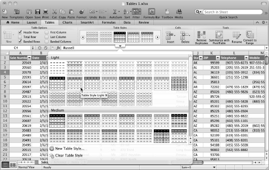
   Figure 10–2. You can format a table quickly by applying one of Excel's table styles from the Table Styles panel on the Tables tab of the Ribbon. Scroll down the panel to see the other styles.

4. In the Table Options group on the Tables tab of the Ribbon, select the check box for each table style option you want to use:
   
   • Header Row. Select this check box to display the header row. This is almost always useful.
   • Total Row. Select this check box to add a row labeled Total immediately after the table's last row. This is useful when you need to add a total formula or another formula in the last row. To add a formula, click a cell in the Total row, click the pop-up button that appears, then click the formula you want on the pop-up menu (see Figure 10–3).
     

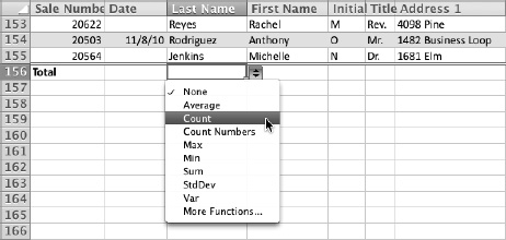
     Figure 10–3. Adding a Total row to a table lets you quickly insert functions in the row's cells. Excel changes the header row to column labels when you scroll down the worksheet.

     TIP: The pop-up menu in the Total row of a table gives you instant access to the most widely used functions in databases—Average, Count, Count Numbers, Max, Min, Sum, StdDev (Standard Deviation), or Var (calculating variance based on a sample). You can also click the More Functions item at the bottom of the pop-up menu to display the Formula Builder, from which you can access the full range of Excel's functions. For example, you can insert the COUNTBLANK() function to count the number of blank cells in a column. You might do this to ensure that a column of essential data contains no blanks.

   • Banded Rows. Select this check box to apply a band of color to every other row. This helps you read the rows of data without your eyes wandering to another row. Some table styles apply banding to the rows automatically.
   • First Column. Select this check box if you want the first column to have different formatting. You may want to do this if the first column contains the main field for identifying each record (for example, a unique number).
   • Last Column: Select this check box if you want the last column to have different formatting. Usually, you'll want this only if the last column contains data that is more important in some way than the data in the other columns.
   • Banded Columns. Select this check box to apply a band of color to every other column. This is sometimes helpful but usually less helpful than banded rows. (Don't use both—the effect is seldom useful.)

When you've finished choosing a style and options for the table, save your work as usual.

Entering Data in a Table

You can enter data in a table either by typing it in directly or by using a data-entry form. In most cases, the data-entry form is the easier option, as you'll see in a moment. You can also connect a table to an external data source, as discussed in the following section.

Entering Data Directly in the Table

A table is essentially an Excel worksheet at heart, so you can enter data in the table by using the standard techniques you've learned in the past few chapters. For example, click a cell, then type data into it; or, if you have the data in another worksheet, copy it and paste it in.

When you enter data in the row immediately after the last row in the table, Excel automatically expands the table to include that row. To add a row within the table, click a cell in the row above which you want to add the new row, then choose Insert Rows from the menu bar. Again, Excel automatically expands the table to include the new row.

To insert a column in the table, click a cell in the column before which you want to add the new column, then choose Insert Columns from the menu bar. Once more, Excel automatically expands the table.

Entering Data Using a Data-Entry Form

Typing directly into the table tends to be awkward, especially when the table contains too many columns to fit in the Excel window with the whole content of each column displayed. When your database has grown beyond a few rows, you can usually enter data more easily by using a data-entry form—a dialog box that Excel automatically tailors to suit your table.

Choose DataForm to display the data-entry form dialog box. Figure 10–4 shows this dialog box, whose title bar shows the name of the worksheet you're using (here, Sales) rather than the word Form.

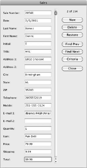
Figure 10–4. The Form dialog box bears the name of the worksheet your table is on (here, Sales) and shows all fields in the order they appear in the header row.

To use the data form, you move to the record you want in one of these ways:

• Create a new record. Click the New button to create a new record in the database. When you type the data in the fields, Excel adds the new record after the last current record in the database.
• Move forward or backward through the records. Click the Find Next button to display the next record, or click the Find Prev button to display the previous record.
• Scroll through the records. Drag the scroll box up or down the scroll bar to move quickly through the records. Click the scroll arrows to move in smaller increments.
• Search for a record. Follow these steps:
  
  1. Click the Criteria button to switch to the criteria view of the form. Excel clears any data in the fields.
  2. Type your search term in the field by which you want to search. For example, to search for your customers in Arizona, type AZ in the State field (assuming your database has this field).
  3. Click the Find Next button to find the next instance, or click the Find Prev button to find the previous instance.

Excel automatically switches the dialog box back to Form view when you search. If you decide you don't need to search after all, click the Form button (which replaces the Criteria button) to return to Form view.

Once you've created or located the record you want to change, type or edit the data in the fields in the data-entry form dialog box. Excel enters it in the columns for you.

When you've finished using the Form dialog box, click the Close button to close it.

Connecting a Table to an External Data Source

If you have your data in an external data source, such as a relational database, you can import the data into an Excel table to work with it. You can then refresh the data in the Excel table with the latest data from the database.

Connecting to a Database

To connect to a relational database, such as a Microsoft Access database or an Oracle database, you need to install an Open Database Connectivity (ODBC) driver for Excel. You can then establish the connection, import the data, and refresh it as needed.

Getting and Installing an ODBC Driver

Before you can import data into a table in Excel, you must install an Open Database Connectivity (ODBC) driver. This is a piece of software that enables Excel to connect to the database and pull data out of it.

Microsoft doesn't provide ODBC drivers for Excel for Mac, so you need to get one from a third-party vendor. To find the latest list of compatible ODBC drivers, open your web browser, go to http://www.microsoft.com/mac/, then search for ODBC Excel. At this writing, there are two providers:

• OpenLink Software (http://www.openlinksw.com/)
• actualtechnologies LLC (http://www.actualtech.com/)

Each offers several different ODBC drivers for different types of database, so make sure you get the right one. Normally, you'll want to start by getting the trial version to make sure it does what you need, then pay for the full version. Some trial versions are limited by time; others are limited by the amount of data they'll return. Either way, you'll eventuallyneed to buy the full version.

Establishing a Connection to a Database

To establish a connection to a database, position the active cell on the appropriate worksheet in the workbook you want to use, then choose Data External Data Sources Database to open the dialog box for setting up the connection. Figure 10.5 shows the iODBC Data Source Chooser dialog box, which you use to establish a connection using OpenLink Software's ODBC driver.

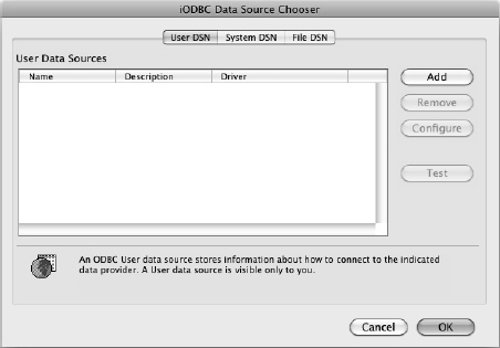
Figure 10–5. Choose your database in the dialog box for the ODBC driver you installed. This screen shows the iODBC Data Source Chooser dialog box.

Use the controls in the dialog box to specify the connection to the data source. The specifics depend on the ODBC driver you're using.

When you have set up the connection, click the Return Data button. Excel displays the Returning External Data to Microsoft Excel dialog box (see Figure 10–6). In this dialog box, you can choose where to place the data that the connection returns:

• Existing sheet. To put the data on an existing worksheet, select this option button, then click the cell you want to use as the upper-left corner of the range. You can click the Collapse Dialog button to get the Returning External Data to Microsoft Excel dialog box out of the way if necessary, but usually it's easy enough just to work around it.
• New sheet. Select this option button if you want to put the data on a new sheet. Excel creates this sheet for you and starts inserting the data at cell A1.
• PivotTable. Select this option button if you want to create a PivotTable from the data. This option button is available only for some types of database connections. (PivotTables are discussed in Chapter 12.)

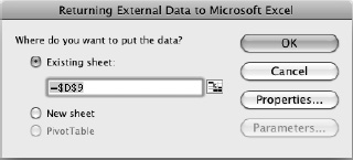
Figure 10–6. In the Returning External Data to Microsoft Excel dialog box, choose whether to put the data on an existing worksheet, on a new worksheet, or in a PivotTable. You can click the Properties button to set the properties for the data returned from the database.

If you need to choose options for how Excel returns the data, click the Properties button in the Returning External Data to Microsoft Excel dialog box to display the External Data Range Properties dialog box (see Figure 10–7). Here you can choose the following options:

• Name. In this text box, type the name you want to give to the external data range. This name is to help you identify the data range; it becomes more important when you use multiple data ranges.
• Query definition. In this box, select the Save query definition check box if you want to save the query; normally, you'll want to do this so you don't have to set it up again. If the query uses a password, you can select the Save password check box to store the password too; you may prefer (or be forced) to enter the password each time for security.
• Refresh control. In this box, select the Prompt for file name on refresh check box if you want Excel to prompt you to enter the file name when you refresh the data. Select the Refresh data on file open check box if you want Excel to refresh the data automatically each time you open the workbook; this is usually helpful if you normally want to work with the latest data. Select the Remove external data from worksheet before saving check box if you want Excel to remove the external data from the workbook when you save it—for example, because you're using the workbook to manipulate data you don't want others to see in it.
• Data layout. In the top part of this box, select the Include field names check box and the Include Row Numbers check box if you want to include these items, as is usually helpful. Select the Adjust column width check box if you want Excel to adjust the column width to fit the data. Select the Import HTML table(s) only check box if you want to import only tables when importing from an HTML data source.
• If the number of rows in the data range changes upon refresh. In this area of the Data layout box, select the appropriate option button: “Insert cells for new data, delete unused cells,” “Insert entire rows for new data, clear unused cells,” or “Overwrite existing cells with new data, clear unused cells.” Normally, the “Insert cells for new data, delete unused cells” option button is the best choice.
• Fill down formulas in columns adjacent to data. Select this check box if you want Excel to automatically fill in formulas down the cells of columns next to the data—for example, to continue a SUM formula you've entered.
• Use Table. Select this check box to have Excel put the external data in a table. This is what you'll usually want.

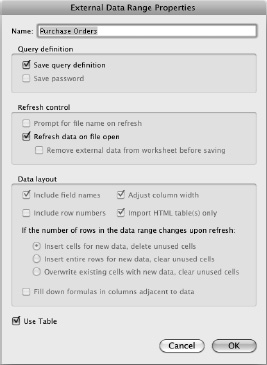
Figure 10–7. In the External Data Range Properties dialog box, name the connection, choose whether to save the query definition, decide when to refresh the data, and choose the layout to use.

When you've finished choosing options in the External Data Range Properties dialog box, click the OK button to close it and return to the Returning External Data to Microsoft Excel dialog box. Then click the OK button to close this dialog box. Excel brings in the data from the data source.

Refreshing the Data from a Database

If you've set the table to update the data from the database automatically at intervals or when you open the workbook, Excel takes care of the refreshing. If you've set the table for manual refreshing, or if you need to pull the latest data into the table right this moment, you can refresh the table manually by using the commands on the Data External Data Sources Refresh menu. Click the Refresh All command to refresh all the tables, or click the Refresh Data command to refresh just the data in the current table.

If a refresh seems to be taking too long, choose Data External Data Sources Refresh Cancel Refresh to cancel it.

Importing Data from a FileMaker Pro Database

If you need to pull data from a FileMaker Pro database into a table, choose Data External Data Sources FileMaker to launch the FileMaker Pro Import Wizard. Follow through the steps of this Wizard as discussed in the section “Importing Data from a FileMaker Pro Database” in Chapter 1.

Resizing a Table

When you've created a table, Excel normally resizes it for you automatically when you add or delete rows or columns. For example, when you add a record by using the Form dialog box, Excel expands the table to include it.

Excel also expands the table automatically if you add data to the row after the current last row in a table that doesn't have a Total row. Excel calls this feature Table AutoExpansion. If you don't want Excel to do this, click the AutoCorrect actions button that appears below and to the right of the first cell in the added row, then click Undo Table AutoExpansion (see Figure 10–8). Click the actions button again, then click Stop Automatically Expanding Tables.

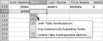
Figure 10–8. You can use the AutoCorrect actions button both to undo Table AutoExpansion and to turn it off.

Sorting a Table by One or More Fields

When you need to examine the data in your table, it's often useful to sort it. Excel lets you sort a table either quickly by a single field or by using multiple fields.

Sorting Quickly by a Single Field

To sort a table by a single field, click any cell in the column you want to sort by, then choose Data Sort & Filter Sort, clicking the main part of the Sort button. This produces a sort in ascending order (A to Z, low values to high values, early dates to later dates, and so on). To reverse the sort to descending order, click the main part of the Sort button again.

After you sort, the table remains sorted that way until you change it.

Sorting a Table by Multiple Fields

Often, it's useful to sort your table by two or more fields at the same time. For example, in a customer database, you may need to sort your customers first by state and then by city within the state.

To sort by multiple fields, follow these steps:

1. Choose Data Sort & Filter Sort Custom Sort to display the Sort dialog box. Figure 10–9 shows the Sort dialog box with two criteria entered and a third criterion under way.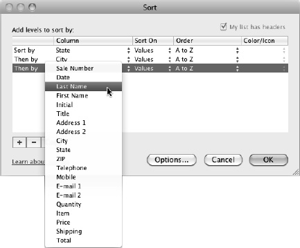
   

   Figure 10–9. In the Sort dialog box, you can set up exactly the sort criteria you need to identify data in your database.

2. Set up your first sort criterion using the controls on the first row of the main part of the Sort dialog box. Follow these steps:
   
   1. Open the Column pop-up menu in the Sort by row, then click the column you want to sort by first. For example, click the State column.
   2. Open the Sort On pop-up menu in the same row, then click what you want to sort by: Values, Cell Color, Font Color, or Cell Icon. In most cases, you'll want to use Values, but the other three items are useful for tables to which you've applied conditional formatting.
   3. Open the Order pop-up menu on the same row, then click the sort order you want. If you choose Values in the Sort On pop-up menu, you can choose A to Z for an ascending sort, Z to A for a descending sort, or Custom List. Choosing Custom List opens the Custom List dialog box, which you can use to choose a custom list by which to sort the results. For example, you could use a custom list of your company's products or offices to sort the database into a custom order rather than being restricted to ascending or descending order.
   4. If you need the sort to be case sensitive (so that “smith” appears before “Smith,” and so on), click the Options button. In the Sort Options dialog box (see Figure 10–10), select the Case Sensitive check box, then click the OK button.
      

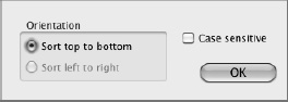
      Figure 10–10. Select the Case sensitive check box in the Sort Options dialog box if you want to treat lowercase letters differently than their uppercase versions.

3. Click the Add (+) button to add a second line of controls to the main part of the Sort dialog box.
4. Set up the criterion for the second-level sort on the Then By line using the same technique. For example, set up a second-level sort using the City column in the database.
5. Set up any other criteria needed by repeating steps 3 and 4.
6. Click the OK button to close the Sort dialog box. Excel sorts the data using the criteria you specified.

Identifying and Removing Duplicate Records in a Table

When you've created a large table, you may need to check it for duplicate records and remove those you find. Excel provides a Remove Duplicates feature that saves you having to comb the records by hand.

To remove duplicate records from a table, follow these steps:

1. Click any cell in the table.
2. Choose Tables Tools Remove Duplicates from the Ribbon or Data Table Tools Remove Duplicates from the menu bar to display the window shown in Figure 10–11.
   
   

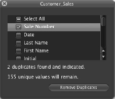
   Figure 10–11. Use this window to locate duplicate values in columns that should contain only unique values. The window's title bar shows the name of the data table.

3. If the Select All check box contains a check mark, click the check box to remove the check mark, and clear all the check boxes in the Columns box.
4. Select the check box for each column you want to check for duplicates. The readout at the bottom of the dialog box shows the number of duplicates.

   TIP: Normally, it's best to check a single column at a time for duplicate values. Make sure that the column is one that must contain a unique value.

5. Click the Remove Duplicates button if you want to remove the duplicates.
6. Repeat the process with another field if necessary.
7. When you have finished removing duplicates, click the  button at the left end of the title bar to close the window.

Filtering a Table

When you need to find records in a table that match the terms you specify, you can filter it. Filtering makes Excel display only the records that match your search terms, hiding all the other records.

To make filtering easy, Excel provides a feature named AutoFilter. To use AutoFilter, follow these steps:

1. Click a cell in the table.
2. Click the Data tab of the Ribbon to display its contents.
3. In the Sort & Filter group, make sure that the Filter button is selected so that it looks pushed in; if not, click the main part of the button. Excel normally selects the Filter button when you create a table, so this button should be pushed in unless you've turned filtering off. Selecting this button makes Excel display a pop-up button on each column heading in the table.
4. On the column you want to use for filtering, click the pop-up button to display the AutoFilter window (shown on the left in Figure 10–12). The AutoFilter window's title bar shows the name of the field you clicked.
   

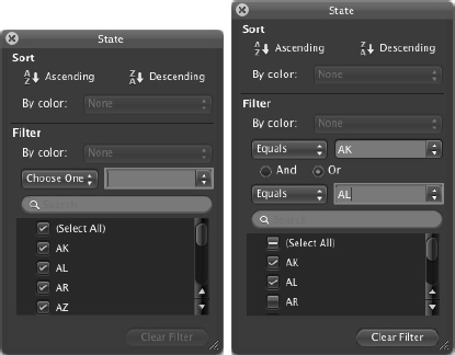
   Figure 10–12. To apply filtering, click the pop-up arrow on a column heading to display the AutoFilter window (left). In the Filter area, open the first pop-up menu, and choose the comparison you want (right). You can then add further comparisons as needed.

5. Click the type of sorting or filtering you want to apply:
   
   • Sort. Click the type of sort you want to apply. Normally, you'll want to click either the Ascending button or the Descending button. But if your data table uses colors, you can sort by color instead—just choose the color in the By color pop-up menu in the Sort area.
   • Filter. If you want to filter the table by color, choose the color in the By color pop-up menu. Otherwise, open the pop-up menu that appears as Choose One in the left part of Figure 10–12, then choose the comparison from it. For example, choose Equals to set a filter that picks particular states, or choose Begins With to set a filter that selects cities that start with text you specify. Use the fields in the Custom AutoFilter window to set up the rest of the comparison; the right screen in Figure 10–12 shows an example that filters by Equals AK or Equals AL, returning the records that have the state AK or the state AL.

When you've specified the details of the filter, Excel applies it to the table and reduces the display to those rows that match the filter. Excel displays a filter symbol in place of the drop-down button on the column that contains the filtering (as on the State column heading in Figure 10–13).

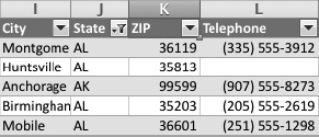
Figure 10–13. The filter symbol (shown on the State column heading here) indicates that you're filtering the table by that column.

To remove filtering from a single column, click the filter symbol on the column heading, then click the Clear Filter button in the AutoFilter window.

To remove filtering from the table as a whole, choose Data Sort & Filter Filter, deselecting the Filter button in the Sort &Filter group.