Viewing Your Workbooks

Excel offers two views for working in your workbooks:

• Normal view. This is the view in which workbooks normally open and it's the one in which you'll do most of your data entry, formatting, and reviewing. Normal view is the view in which you've seen Excel so far in this chapter.
• Page Layout view. This view shows your worksheets as they'll look when laid out on paper. You use it to adjust the page setup. You'll learn how to do this in the section “Formatting Pages” in Chapter 4.

To switch the view, click the Normal View button or the Page Layout View button at the left end of the status bar (see Figure 1–31) or choose View Normal or View Page Layout from the menu bar.

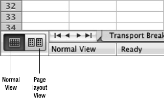
Figure 1–31. Use the View buttons at the left end of the status bar to change views quickly.

Splitting the Window to View Separate Parts of a Worksheet

Often, it's useful to be able to see two parts of a worksheet at the same time—for example, to make sure your notes correctly describe your data or when you're copying information from one part to another.

When you need to see two parts of the worksheet in the same window, you can split the window either horizontally or vertically. To do so, you use the horizontal split box at the right end of the horizontal scroll bar, the vertical split box at the top end of the vertical scroll bar, or the Split button in the Window group of the Layout tab of the Ribbon (see Figure 1–32).

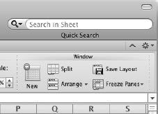
Figure 1–32. The Window group on the Layout tab of the Ribbon contains several essential commands, but most of the button names appear only when the Excel window is very wide.

Double-click the horizontal split box to split the window horizontally above the active cell, or double-click the vertical split box to split the window vertically to the left of the active cell. If the active cell isn't in the right place for splitting, click the horizontal split box or the vertical split box, and then drag it until the split bar appears where you want the split.

If you want to split the window into four panes, you can also split it in the other dimension. For example, if you've already split the window horizontally, now split it vertically as well. Figure 1–33 shows the Excel window split into four panes.

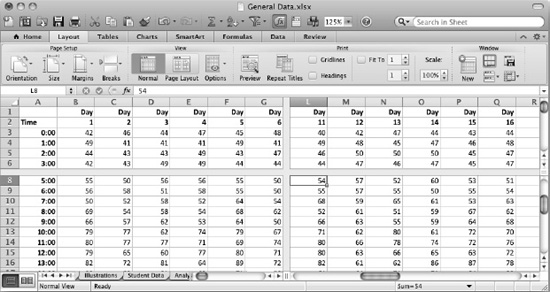
Figure 1–33. Split the Excel window into two or four panes when you need to work in separate areas of the worksheet at the same time.

Once you split the window, you get a separate scroll bar in each part, so you can scroll the panes separately to display whichever areas of the worksheet you need.

To reposition the split, click the split bar, and drag it to where you want it. If you've split the window into four panes, you can resize all four panes at once by clicking where the split bars cross and then dragging.

To remove the split, either double-click the split bar or click and drag it all the way to the left of the screen or all the way to the top. You can also choose Layout Window Split from the Ribbon or Window Remove Split from the menu bar.

Opening Extra Windows to Show Other Parts of a Workbook

Instead of splitting a window, you can open one or more extra windows to show other parts of the workbook.

Choose Layout Window New from the Ribbon or Window New Window from the menu bar to open a new window in the active workbook. Excel distinguishes the windows by adding :1 to the name of the first and :2 to the name of the second—for example, General Data.xlsx:1 and General Data.xlsx:2.

Changing the Window and Arranging Open Windows

The easiest way to change the window you're working in is to click the window you want to use—either click the window itself (if you can see it) or click its button on the Taskbar. You can also choose to open the Window menu on the menu bar and then click the window in the list at the bottom.

When you've opened several windows, you can arrange them using standard Mac OS X techniques, such as by dragging them to the size and position you want. You can also use Excel's Arrange Windows dialog box or Arrange pop-up menu to place the windows.

To position windows using the Arrange Windows dialog box, follow these steps:

1. Choose Window Arrange from the menu bar or Layout Window Arrange Arrange Windows from the Ribbon to display the Arrange Windows dialog box (see Figure 1–34).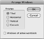
   

   Figure 1–34. Use the Arrange Windows dialog box to tile or otherwise arrange all Excel windows or only those from the active workbook.

2. Click the option button for the arrangement you want:
   • Tiled. Select this option button to make Excel resize all the non-minimized windows to roughly even sizes so they fit in the Excel window. If you have several windows open, tiling may make them too small to work in, but it's good for seeing which windows are open and closing those you don't need.
   • Horizontal. Select this option button to arrange all the windows horizontally in the Excel window. This arrangement works well for two windows in which the data is laid out in rows rather than columns.
   • Vertical. Select this option button to arrange all the windows vertically in the Excel window. This arrangement works well for two windows in which the data is laid out in columns rather than rows.
   • Cascade. Select this option button to arrange the windows in a stack so you can see each one's title bar. This arrangement is useful for picking the window you want out of many open windows.
3. To arrange only the windows of the active workbook, select the Windows of active workbook check box. This option is good for the Horizontal and Vertical arrangements.
4. Click the OK button to close the Arrange Windows dialog box. Excel arranges the windows as you chose.

To arrange windows quickly using the Arrange pop-up menu, choose Layout Window Arrange, and then click either Vertical or Cascade on the pop-up menu, as needed. You can also click the Arrange Windows item to display the Arrange Windows dialog box.

Zooming to Show the Data You Need to See

To make a worksheet's data easier to read, you can zoom in. Or if you need to see more of a worksheet at once, you can zoom out.

The easiest way to zoom in or out is by opening the Zoom pop-up menu on the Standard toolbar and then clicking one of the items on it: 200%, 150%, 125%, 100%, 75%, 50%, 25%, Selection, or (in Page Layout view only) One Page.

You can set a custom view percentage by clicking the Zoom box or opening the Zoom pop-up menu, typing the percentage you want, and then pressing Return.

When you need to zoom just the right amount to display a particular area of the worksheet as large as it will fit in the window, select the area, open the Zoom pop-up menu, and then click Selection.

Freezing Rows and Columns So They Stay Onscreen

To keep your data headings onscreen when you scroll down or to the right on a large worksheet, you can freeze the heading rows and columns in place. For example, if you have headings in column A and row 1, you can freeze column A and row 1 so they remain onscreen.

You can quickly freeze the first column, the top row, or your choice of rows and columns:

• Freeze the first column. Choose Layout Window Freeze Panes Freeze First Column from the Ribbon.
• Freeze the first row. Choose Layout Window Freeze Panes Freeze Top Row from the Ribbon.
• Freeze your choice of rows and columns. Click the cell below the row and to the right of the column you want to freeze. For example, to freeze the top two rows and column A, select cell B3. Then choose Layout Window Freeze Panes Freeze Panes from the Ribbon or Window Freeze Panes from the menu bar.

Excel displays a gray line along the gridlines of the frozen cells. Once you've applied the freeze, the frozen columns and rows don't move when you scroll down or to the right. Figure 1–35 shows a worksheet with rows 1 and 2 and column A frozen.

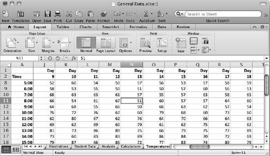
Figure 1–35. Freeze the heading rows and columns to keep them in place when you scroll down or across the worksheet.

When you no longer need the freezing, choose Layout Window Freeze Panes Unfreeze from the Ribbon or Window Unfreeze Panes from the menu bar to remove it.