
Documenting Your Workbooks
When you're creating a workbook and entering data in it, you'll probably be clear about which data is which, why you're laying the data out in the way you've chosen, and why you've used particular types of charts or decided to construct formulas in an idiosyncratic way.
But someone else who opens your workbooks may not intuitively grasp how you've done things. So when you create a workbook you plan to share with others, or when you prepare a workbook for sharing, it's a good idea to document the workbook. This can save you time, bewilderment, and any number of infuriating questions in the days, weeks, or months to come.
Excel provides three main tools for documenting your workbooks:
- Text in cells
- Comments attached to cells
- Data-validation tools
We'll look at each of these tools in turn.
Adding Explanatory Text to Workbooks
The most straightforward way to document a workbook is to enter text in the cells. You already know how to do this, so the only issue is what text to enter and how vigorously to format it so that nobody can miss it.
As a general rule, you'll save yourself grief by explaining more than seems strictly necessary. For example, it should perhaps be obvious that the worksheet named Western Region Sales 2011 contains sales results for the Western Region in 2011—but you should probably put that information in a cell at the top of the worksheet as well for anyone who doesn't look at the worksheet tab. Similarly, even if the formulas you've used are standard and straightforward, it's a good idea to make clear how the figures they show are derived. For this, you can either use text in nearby cells or attach comments to the cells themselves (as discussed in the next section).
TIP: For a complex workbook that contains many worksheets, add a Summary worksheet or Introduction worksheet at the beginning. On this worksheet, state the workbook's purpose and enter a list of the worksheets and what they contain. You may also want to note who's supposed—or permitted—to do what with the workbook. For example, managers must fill in their budget figures, while VPs are to look at the Executive Overview worksheet and approve the figures there but not mess with any other worksheets. You can add macro buttons to the Summary worksheet to display particular worksheets, providing an easy way to navigate the workbook. (See Chapter 14 for coverage of macros.)
Adding Comments to Cells
Entering explanatory text directly in cells makes it easy to see, but you may also want to add information using comments. A comment is text attached to a cell. Excel displays a comment indicator in the cell to indicate a comment is attached; when you hold the mouse pointer over the cell, the comment appears in a balloon. You can also display all the comment balloons on a worksheet, and rearrange them if they overlap.
Adding a Comment
To add a comment to a cell, follow these steps:
- Make active the cell to which you want to add the comment.
- Choose Review
 Comments New from the Ribbon or Insert New Comment from the menu bar. Excel displays the comment marker and a red triangle in the upper-right corner of the cell, opens a comment balloon, and enters your user name in the balloon in boldface.
TIP: Excel enters your user name (as set in Excel's General preferences pane) in each comment for you, but you can edit the name if necessary, or simply delete it. To make your comments more readable or dramatic, you can apply text formatting to them. For example, click the Bold button or press Cmd+B to make selected text bold.
- Type the text of the comment. Figure 13–7 shows an example.
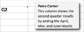
Figure 13–7. The red triangle at the upper-right corner of the Q2 cell here is the comment marker. Type or paste the text for the comment in the comment balloon.
- When you have finished creating the comment, click anywhere in the worksheet to move the focus from the comment.
NOTE: If the comment indicator doesn't appear in the cell, Excel is set to hide comments and indicators. Choose Review ![]() Comments
Comments ![]() Show All from the Ribbon to turn on the display of comments.
Show All from the Ribbon to turn on the display of comments.
TIP: When you're working with multiple versions of the same worksheet, you may need to paste comments from one worksheet to another. You can do this easily by using the Paste Special command. Select the range that contains the comments, then copy it to the Clipboard as usual (for example, press Cmd+C). Next click the cell at the upper-left corner of the destination range, choose Home ![]() Edit
Edit ![]() Paste
Paste ![]() Paste Special, select the Comments option button in the Paste area, then click the OK button.
Paste Special, select the Comments option button in the Paste area, then click the OK button.
Viewing Comments
Normally, Excel displays only the comment markers in a worksheet. To view a comment, you hold the mouse pointer over a cell that contains a comment, and Excel displays the comment in a balloon. You can also click the cell and then choose Review ![]() Comments
Comments ![]() Show from the Ribbon to display a comment and keep it displayed while you move to other parts of the worksheet.
Show from the Ribbon to display a comment and keep it displayed while you move to other parts of the worksheet.
If you want to display all the comments, choose Review ![]() Comments
Comments ![]() Show All from the Ribbon or View
Show All from the Ribbon or View ![]() Comments from the menu bar.
Comments from the menu bar.
To select the next comment, choose Review ![]() Comments
Comments ![]() Next. To select the previous comment, choose Review
Next. To select the previous comment, choose Review ![]() Comments
Comments ![]() Previous.
Previous.
Deleting Comments
To delete a comment, follow these steps:
- Select the comment. You can either click the cell that contains the comment or choose Review Comments Next or Review Comments Previous to select the comment.
- Give the Delete command. Either press the Delete key or choose Review Comments Delete.
TIP: You can edit a comment by Ctrl-clicking or right-clicking a commented cell and then clicking Edit Comment. Similarly, you can delete a comment by Ctrl-clicking or right-clicking a commented cell, and then clicking Delete Comment.
Adding Information with Data Validation
As you saw in the section “Checking Input with Data Validation” in Chapter 4, you can apply data-validation formatting to a cell to make sure that the value the user enters in it meets your requirements. For example, you can use data validation to ensure that the value the user enters is between 250 and 1000 (inclusive) and to display an error alert message box if it's not.
You can use data validation to add information to your worksheets in two ways:
- Display an input message. On the Input Message tab of the Data Validation dialog box, select the Show input message when cell is selected check box, then type the title in the Title text box and the message in the Input message text box. When the user selects the cell, Excel displays a balloon containing the input message. This works like an automated comment and can be a great way of providing focused guidance on how to use a workbook.
- Display an error alert. On the Error Alert tab of the Data Validation dialog box, select the Show error alert after invalid data is entered check box, then specify the title and error message to include in the dialog box. You can also use this feature to provide detailed instructions for users of your workbooks.