Creating a Collapsible Worksheet by Outlining It

Worksheets that contain many columns or rows of data can become hard to navigate even if you freeze the headings on screen the way you learned in Chapter 1. To make navigation easier, you can use Excel's outlining feature to create a collapsible worksheet, and then expand only those sections you need to see at any particular time. Figure 3–17 shows a worksheet containing an outline with some rows and columns expanded and others collapsed.

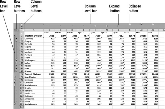
Figure 3–17. Use Excel's outline features to create a worksheet that you can collapse and expand to show only the sections you need.

Outlining works best for worksheets whose data is arranged in a structure or hierarchy. You can create up to eight levels for rows and eight levels for columns, giving you fine control over the outlines.

You can have Excel create an outline automatically for you from the structure it detects in a worksheet you've laid out with formulas. This is often the best way to start. If you find the automatic outline isn't what you need, you can create an outline manually instead, putting the levels exactly where you want them.

Having Excel Create an Outline Automatically

To have Excel create an outline automatically, you must set up the structure of the worksheet with the formulas in place. Excel uses the formulas to determine the hierarchy of the outline, so if the formulas aren't there, outlining doesn't work. You don't need to enter all the rows and columns of data—just those that contain the formulas and enough of the data rows and columns for the formulas to refer to.

The left screen in Figure 3–18 shows the beginning of a worksheet structured with formulas that will produce an outline. Here's what you can see:

• The leftmost column (column A) contains the divisions, states, and city offices of a large and nefarious organization that we'll allow to remain nameless. You can see the Western Division (which contains California, Oregon, Washington, Idaho, Nevada, Utah, and Arizona) and the Central Division (which includes New Mexico, Montana, Colorado, and various states you can't see).
• Each state contains just a couple of the offices to get the structure right. Once the structure is in place, you can add the extra rows needed.
• Each state's row contains a SUM() formula that adds up the results of the city offices. For example, the California row contains the formula =SUM(B4:B5) in cell B3, adding the rich pickings from Bakersfield and Chico.
• Each division's row contains a SUM() formula that adds up the results of the division's states. For example, the Western Division row contains the formula =SUM(B3,B6,B9,B12,B15,B18,B22) in cell B2, adding the results from California, Oregon, and so on.

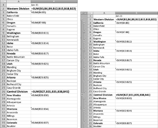
Figure 3–18. By setting up a worksheet with a hierarchy of formulas (left), you can use Excel's automatic outlining feature to create an outline based on the formulas (right).

When you've got the formulas in place, choose Data Group & Outline Group Auto Outline from the Ribbon or Data Group and Outline Auto Outline from the menu bar to create the outline automatically. The right screen in Figure 3–18 shows the same range of data turned into an outline with three levels. You can click one of the – signs in the outlining bar on the left to collapse a section, and click the + sign that replaces the – sign to expand a section again.

If the outline turns out the way you want it, you can enter the remaining formulas and data. In many cases, you'll be able to use the AutoFill feature (discussed in Chapter 1) to automatically insert the formulas in a row or column based on an existing formula.

If the automatic outline doesn't suit you, try changing the settings for automatic outlining, as discussed next. Alternatively, clear the outline by choosing Data Group & Outline Ungroup Clear Outline from the Ribbon or Data Group and Outline Clear Outline from the menu bar. You can then create your outline manually, as discussed in the section after next.

Changing the Settings for Outlining

To change the settings that Excel uses for outlining, follow these steps:

1. Choose the data range:
   • To change an existing outline, click any cell in the outline.
   • To create a new outline, select the data range.
2. Choose Data Group and Outline Settings from the menu bar to display the Settings dialog box (see Figure 3–19).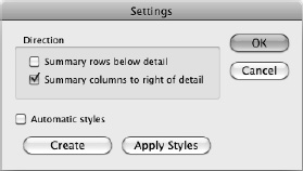
   

   Figure 3–19. Use the Settings dialog box to control the way Excel creates an automatic outline from your worksheet.

3. In the Direction box, select the Summary rows below detail check box if the summary rows are below the detail rows. Select the Summary columns to right of detail check box if the worksheet uses summary columns that appear to the right of the columns they summarize.
4. Select the Automatic styles check box if you want Excel to automatically apply styles to the outline to differentiate the different outline levels. Excel applies the RowLevel_1 style to the first level of rows, the RowLevel_2 style to the second level of rows, and so on. For the columns, Excel uses styles named ColLevel_1, ColLevel_2, and so on.
5. Click the command button to close the Settings dialog box and take the action you want:
   • Create. Click this button to create a new outline.
   • Apply Styles. Click this button to apply styles to an existing outline. You'll need to have selected the Automatic styles check box.
   • OK. Click this button to apply the Direction settings you've chosen to an existing outline.

Creating an Outline Manually

Often, it's not convenient to build the structure of a worksheet fully so that Excel can outline it automatically. In these cases, create the outline manually by using the Group command. You can also use the Group command (and its counterpart, Ungroup) to adjust an outline Excel has created for you.

Grouping Rows or Columns

To group rows or columns, follow these steps:

1. Select cells in the rows or columns you want to group. For example:
   • To group rows 4 and 5 under row 3, select cells in rows 4 and 5.
   • To group columns B, C, and D under column E, select cells in columns B, C, and D.

     TIP: You can speed up the process of grouping or ungrouping rows or columns by selecting entire rows or entire columns rather than just cells in them. When you do this, Excel doesn't display the Group dialog box or the Ungroup dialog box, because it can tell from the selection whether it's rows or columns you want to group or ungroup.

2. Choose Data Group & Outline Group from the Ribbon (clicking the main part of the Group button rather than its pop-up button) or Data Group and Outline Group from the menu bar to display the Group dialog box (shown on the left in Figure 3–20).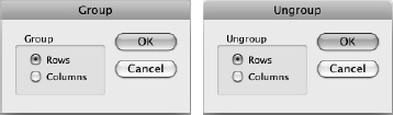
   

   Figure 3–20. In the Group dialog box (left) or the Ungroup dialog box (right), select the Rows option button or the Columns option button, as appropriate.

3. Select the Rows option button if you want to group by rows. Select the Columns option button if you want to group by columns.
4. Click the OK button to close the Group dialog box. Excel applies the grouping.

Repeat this procedure to create more groups as needed. For example, in the worksheet I showed you earlier, you would first group the cities under their states, and then group the states under their divisions.

Ungrouping Rows or Columns

To ungroup rows or columns, follow these steps:

1. Select the range you want to ungroup.
2. Choose Data Group & Outline Ungroup from the Ribbon (clicking the main part of the Ungroup button rather than its pop-up button) or Data Group and Outline Ungroup from the menu bar to display the Ungroup dialog box (shown on the right in Figure 3–20).
3. Select the Rows option button or the Columns option button, as appropriate.
4. Click the OK button to close the Ungroup dialog box and remove the grouping.

Expanding and Collapsing an Outline

When you have created the outline, you can expand it or collapse it so it shows exactly what you need to see.

Click the Column Level button for the column level you want to see. For example, click the Column Level 2 button to display all the second-level columns.

Click the Row Level button for the row level you want to see. For example, click the Row Level 3 button to display all of the third-level rows.

Click the + button to expand a collapsed section of rows or columns or the – button to collapse an expanded section.

Updating the Outline After Adding or Deleting Rows or Columns

After you add or delete rows or columns within the outlined area of a worksheet, you need to update the outline. Follow these steps:

1. Place the active cell anywhere in the outlined area.
2. Choose Data Group & Outline Group Auto Outline from the Ribbon or Data Group and Outline Auto Outline from the menu bar. Excel displays the untitled dialog box shown in Figure 3–21.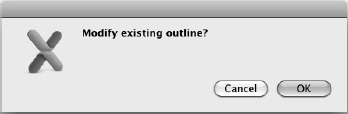
   

   Figure 3–21. Click the OK button in this dialog box to update the outline with details of the rows or columns you've added or deleted.

3. Click the OK button. Excel updates the outline.

Remove an Outline

To remove outlining from a worksheet, choose Data Group & Outline Ungroup Clear Outline.