Formatting Cells and Ranges

In Excel, you can format cells in a wide variety of ways—everything from choosing how to display the borders and background to controlling how Excel represents the text you enter in the cell. This section shows you how the most useful kinds of formatting work and how to apply them.

Each cell comes with basic formatting applied to it—the font and font size to use and usually the General number format, which you'll meet shortly. So when you create a new workbook and start entering data in it, Excel displays the data in a normal-size font.

Understanding the Three Main Tools for Applying Formatting

Excel gives you three main tools for applying formatting to cells and ranges:

• Formatting Toolbar. If you display this toolbar (choose View Toolbars Formatting from the menu bar), you can quickly apply some of the most widely used formatting. Figure 4–5 shows the Formatting toolbar (displayed undocked so you can see it more easily) with its controls labeled.

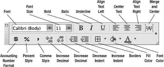
Figure 4–5. The Formatting toolbar is often the easiest way to apply widely used formatting.

• Home tab of the Ribbon. The Font group provides widely used font formatting; the Alignment group offers horizontal and vertical alignment, orientation, indentation, wrapping, and merging; and the Number group gives you a quick way to apply essential number formatting. Figure 4–6 shows the Font group with its controls labeled. Figure 4–7 shows the Alignment group and Number group with their controls labeled.

Figure 4–6. You can quickly apply essential font formatting, borders, and fills from the Font group on the Home tab of the Ribbon.

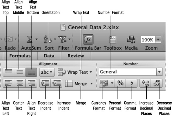
Figure 4–7. From the Alignment group on the Home tab of the Ribbon, you can set horizontal and vertical alignment, orientation, and wrapping. From the Number group, you can apply number formatting.

• Format Cells dialog box. When you need to apply formatting types that don't appear on the Standard toolbar or on the Home tab of the Ribbon, open the Format Cells dialog box and work on its six tabs, which you'll meet later in this chapter. The easiest way to display the Format Cells dialog box is to Ctrl+click or right-click a cell or a selection and then click Format Cells on the context menu. You can also open the Format Cells dialog box by pressing Cmd+1 or choosing Format Cells from the menu bar.

Controlling How Data Appears by Applying Number Formatting

When you enter a number in a cell, Excel displays it according to the number formatting applied to that cell. For example, if you enter 39250 in a cell formatted with General formatting, Excel displays it as 39250. If the cell has Currency formatting, Excel displays a value such as $39,250.00 (depending on the details of the format). And if the cell has Date formatting, Excel displays a date such as 18 June 2011 (again, depending on the details of the format). In each case, the number stored in the cell remains the same—so if you change the cell's formatting to a different type, the way that Excel displays the data changes to match.

Table 4–1 explains Excel's number formats and tells you the keyboard shortcuts for applying them. You can also apply number formatting by using the buttons on the Standard toolbar, the Number Format pop-up menu and buttons in the Number group of the Home tab of the Ribbon, and the Number tab of the Format Cells dialog box (see Figure 4–8).

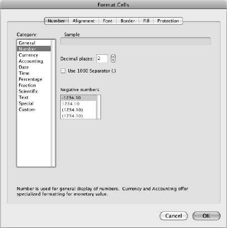
Figure 4–8. Use the Number tab of the Format Cells dialog box when you need access to the full range of number formatting.

Table 4–1. Excel's Number Formats

UNDERSTANDING HOW EXCEL STORES DATES AND TIMES

To create a custom number format of your own, follow these steps:

1. Select a cell that contains the right kind of data. For example, if you want to create a custom date format, select a cell with Date formatting and a date entered in it.
2. Open the Format Cells dialog box by pressing Cmd+1.
3. Click the Number tab if it's not displayed at first.
4. In the Category list box, click the Custom item. Excel displays the controls for creating a custom format (see Figure 4–9). Your sample data appears in the Sample box at the top.
   

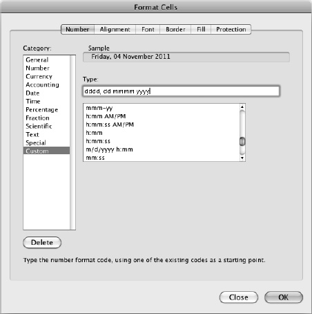
   Figure 4–9. You can create custom number formats by typing them in the Type text box on the Number tab of the Format Cells dialog box. Click the most similar format in the list box to give yourself a head start.

5. Scroll down the list box until you find the format that's closest to the format you want to create, then click that format. Excel adds the codes for the format to the Type text box and shows the sample data in that format.
6. Edit the format so that the sample data appears the way you want it (see the instructions after this list).
7. Click the OK button to close the Format Cells dialog box.

To create a custom format, you enter format codes telling Excel how to display the information. A custom format can contain a single format, like the date format shown in Figure 4–9, but you can include up to four different formats, separated by semicolons:

• First format. How to display positive numbers.
• Second format. How to display negative numbers.
• Third format. How to display zero values.
• Fourth format. How to display text.

Table 4–2 explains the codes for creating custom number formats.

Table 4–2. Codes for Creating Custom Number Formats

Setting the Workbook's Overall Look by Applying a Theme

To control the overall look of a workbook, apply a suitable theme to it by choosing Home Themes Themes and then clicking the theme you want on the Themes panel.

The theme applies a set of colors and a pair of fonts to the workbook. After applying the theme, you can change the colors or fonts by using the Colors pop-up menu or the Fonts pop-up menu in the Themes group on the Home tab of the Ribbon.

Choosing How to Align Cell Contents

You can quickly align the contents of cells by using the buttons in the Alignment group on the Home tab of the Ribbon or the controls on the Alignment tab of the Format Cells dialog box (see Figure 4–10):

• Horizontal alignment. You can align the text Left, Center, Right, or Justify; apply General alignment, which depends on the data type (left for text, right for numbers); choose Center Across Selection to center the text across multiple cells; or choose Distributed (Indent) to distribute the text across the cell (using wider spaces between words).

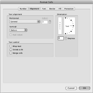
Figure 4–10. The Alignment tab of the Format Cells dialog box lets you rotate text to precise angles when needed.

• Vertical alignment. You can align text Top, Center, Bottom, or Justify. You can also choose Distributed to distribute the text vertically, which can be useful when you rotate the text so that it runs vertically.
• Rotate text. Use the Orientation box on the Alignment tab of the Format Cells dialog box or the Orientation pop-up menu in the Alignment group.
• Indentation. You can indent the text as far as is needed.
• Wrap. You can wrap the text to make a long entry appear on several lines in a cell rather than disappear where the next cell's contents start. When you wrap text, Excel automatically increases the row height to accommodate the wrapped text. (If you set a specific row height that's less than the height needed to display all the wrapped text, only the text that fits appears in the cell.)
• Shrink to fit. Select this check box on the Alignment tab of the Format Cells dialog box to shrink the text so that it fits in the cell. Shrinking works well when the text is only a bit too big for the cell. If the text is much too big, shrinking makes it too small to read.
• Merge cells. Use the Merge & Center pop-up menu in the Alignment group to merge selected cells together into a single cell. You can also center an entry across a merged cell. In the Format Cells dialog box, you can merge cells by selecting the Merge cells check box on the Alignment tab.

Choosing Font Formatting

You can quickly format the contents of a cell (or the selected part of a cell's contents) by using the controls on the Standard toolbar, the controls in the Font group on the Home tab, or the Font tab of the Format Cells dialog box (see Figure 4–11).

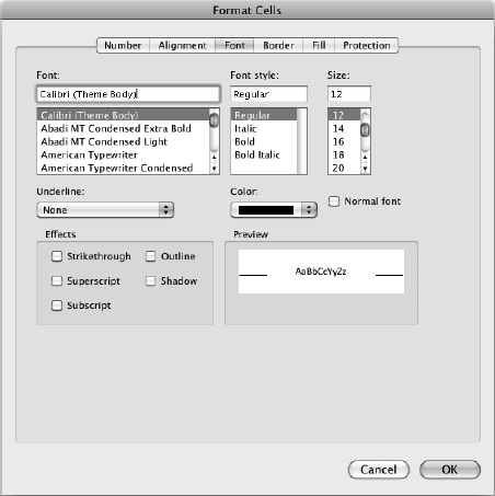
Figure 4–11. Use the Font tab of the Format Cells dialog box when you need a fuller range of font formatting than the Standard toolbar and the Ribbon's Font group provide.

Applying Borders and Fills

To apply borders to a cell, open the Borders pop-up menu in the Font group on the Home tab of the Ribbon, and then click the border type you want (see Figure 4–12).

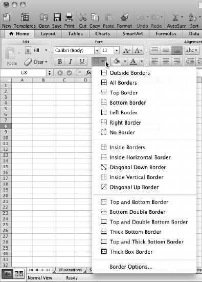
Figure 4–12. You can quickly apply borders from the Borders pop-up menu in the Font group of the Home tab.

For more border options, click the Border Options item at the bottom of the Borders pop-up menu to display the Border tab of the Format Cells dialog box (see Figure 4–13). You can also choose Format Cells from the menu bar (or press Cmd+1) and then click the Border tab. Use the controls on the Border tab to set up the borders you want. For example, to apply a heavy bottom border, click a dark line in the Style box, and then click the Bottom Border button in the Border box. Then click the OK button.

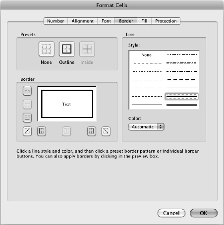
Figure 4–13. Use the Border tab of the Format Cells dialog box when you need to change the line style or color of borders.

To apply a fill, use the Fill Colors pop-up menu in the Font group on the Home tab of the Ribbon or the Fill Colors pop-up menu on the Formatting toolbar, or work on the Fill tab of the Format Cells dialog box.

Applying Protection to Cells

The Protection tab of the Format Cells dialog box contains only two controls:

• Locked. Select this check box to lock a cell against changes.
• Hidden. Select this check box to hide the formula in a cell (the formula's result remains visible).

After selecting either of these check boxes, you must protect the worksheet before the locking or hiding takes effect. You'll learn how to protect a worksheet in the section “Protecting a Worksheet or Workbook” in Chapter 13.