MARK J. P. ANSON, PhD, JD, CPA, CFA, CAIA
President and Executive Director of Nuveen Investment Services
FRANK J. FABOZZI, PhD, CFA, CPA
Professor in the Practice of Finance, Yale School of Management
MOORAD CHOUDHRY, PhD
Head of Treasury, KBC Financial Products, London
REN-RAW CHEN, PhD
Associate Professor of Finance, Rutgers University
Abstract: The total return on a bond, bond portfolio, or bond index is taken into account interest income and any capital gain or loss realized. In the fixed income market, derivative instruments that allow an investor to obtain exposure to the total return of a bond, bond portfolio, or bond index without the actual purchase of the underlying is available. This derivative instrument is a total return swap. Similarly, a total return swap can be used to short the underlying without the need to borrow it.
Keywords: total return swap, total return bond index swap, total return index swap, swap buyer, swap seller, interest rate swap, basis swap, funding leg, synthetic repo
A total return swap is a swap in which one party makes periodic floating rate payments to a counterparty in exchange for the total return realized on a reference asset (or underlying asset). In the fixed income market, reference asset could be a credit-risky bond, a reference portfolio consisting of bonds or loans, or an index representing a sector of the bond market. We first explain how a total return swap can be used when the reference asset is a credit-risky bond and a loan. While these types of total return swaps are more aptly referred to as total return credit swaps, we will simply refer to them as total return swaps. When the bond index consists of a credit risk sector of the bond market, the total return swap is referred to as a total return bond index swap or in this chapter as simply a total return index swap. We will explain how a total return index swap offers asset managers and hedge fund managers greater flexibility in managing a bond portfolio. (For the valuation of fixed income total return swaps, see Chapter 48 of Volume III).
A total return of a reference asset includes all cash flows that flow from it as well as the capital appreciation or depreciation of the reference asset. The floating rate is a reference interest rate (typically the London Interbank Offered Rate [LIBOR]) plus or minus a spread. The party that agrees to make the floating rate payments and receive the total return is referred to as the total return receiver or the swap buyer; the party that agrees to receive the floating rate payments and pay the total return is referred to as the total return payer or swap buyer. Total return swaps are viewed as unfunded credit derivatives, because there is no up-front payment required.
If the total return payer owns the underlying asset, it has transferred its economic exposure to the total return receiver. Effectively, then, the total return payer has a neutral position that typically will earn LIBOR plus a spread. However, the total return payer has only transferred the economic exposure to the total return receiver; it has not transferred the actual asset. The total return payer must continue to fund the underlying asset at its marginal cost of borrowing or at the opportunity cost of investing elsewhere the capital tied up by the reference assets.
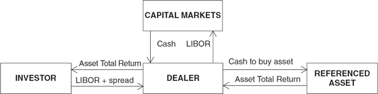
The total return payer may not initially own the reference asset before the swap is transacted. Instead, after the swap is negotiated, the total return payer will purchase the reference asset to hedge its obligations to pay the total return to the total return receiver. In order to purchase the reference asset, the total return payer must borrow capital. This borrowing cost is factored into the floating rate that the total return receiver must pay to the swap seller. Figure 43.1 diagrams how a total return credit swap works.
In Figure 43.1 the dealer raises cash from the capital markets at a funding cost of straight LIBOR. The cash that flows into the dealer from the capital markets flows right out again to purchase the reference asset. The asset provides both interest income and capital gain or loss depending on its price fluctuation. This total return is passed through in its entirety to the investor according to the terms of the total return swap. The investor, in turn, pays the dealer LIBOR plus a spread to fulfill its obligations under the swap.
From the dealer's perspective, all of the cash flows in Figure 43.1 net out to the spread over LIBOR that the dealer receives from the investor. Therefore, the dealer's profit is the spread times the notional amount of the total return swap. Furthermore, the dealer is perfectly hedged. It has no risk position except for the counterparty risk of the investor. Effectively, the dealer receives a spread on a riskless position.
In fact, if the dealer already owns the reference asset on its balance sheet, the total return swap may be viewed as a form of credit protection that offers more risk reduction than a credit default swap. A credit default swap has only one purpose: To protect the investor against default risk. If the issuer of the reference asset defaults, the credit default swap provides a payment. However, if the underlying asset declines in value but no default occurs, the credit protection buyer receives no payment. In contrast, under a total return swap, the reference asset owned by the dealer is protected from declines in value. In effect, the investor acts as a "first loss" position for the dealer because any decline in value of the reference asset must be reimbursed by the investor.
The investor, however, receives the total return on a desired asset in a convenient format. There are several other benefits in using a total return swap as opposed to purchasing a reference asset itself. First, the total return receiver does not have to finance the purchase of the reference asset itself. Instead, the total return receiver pays a fee to the total return payer in return for receiving the total return on the reference asset. Second, the investor can take advantage of the dealer's "best execution" in acquiring the reference asset. Third, the total return receiver can achieve the same economic exposure to a diversified basket of assets in one swap transaction that would otherwise take several cash market transactions to achieve. In this way, a total return swap is a much more efficient means for transacting than via the cash market. Finally, an investor who wants to short a credit-risky asset such as a corporate bond will find it difficult to do so in the market. An investor can do so efficiently by using a total return swap. In this case the investor will use a total return swap in which it is a total return payer.
There is a drawback of a total return swap if an asset manager employs it to obtain credit protection. In a total return swap, the total return receiver is exposed to both credit risk and interest rate risk. For example, the credit spread can decline (resulting in a favorable price movement for the reference asset), but this gain can be offset by a rise in the level of interest rates.
It is worthwhile comparing market conventions for a total return swap to that of an interest rate swap. A plain vanilla or generic interest rate swap involves the exchange of a fixed-rate payment for a floating-rate payment. A basis swap is a special type of interest rate swap in which both parties exchange floating-rate payments based on a different reference interest rate. For example, one party's payments may be based on 3-month LIBOR, while the other parties payment is based on the 6-month Treasury rate. In a total return swap, both parties pay a floating rate.
The quotation convention for a generic interest rate swap and a total return swap differ. In a generic interest rate swap, the fixed-rate payer pays a spread to a Treasury security with the same tenor as the swap and the fixed-rate receiver pays the reference rate flat (that is, no spread or margin). The payment by the fixed-rate receiver (that is, floating rate payer) is referred to as the funding leg. For example, suppose an interest rate swap quote for a 5-year, 3-month LIBOR-based swap is 50. This means that the fixed-rate payer agrees to pay the 5-year Treasury rate that exists at the inception of the swap and the fixed-rate receiver agrees to pay 3-month LIBOR. In contrast, the quote convention for a total return swap is that the total return receiver receives the total return flat and pays the total return payer a interest rate based on a reference rate (typically LIBOR) plus or minus a spread. That is, the funding leg (that is, what the total return receiver pays includes a spread).
Let's illustrate a total return swap where the reference asset is a corporate bond. Consider an asset manager who believes that the fortunes of XYZ Corporation will improve over the next year so that the company's credit spread relative to U.S. Treasury securities will decline. The company has issued a 10-year bond at par with a coupon rate of 9% and therefore the yield is 9%. Suppose at the time of issuance, the 10-year Treasury yield is 6.2%. This means that the credit spread is 280 bps and the asset manager believes it will decrease over the year to less than 280 bps.
The asset manager can express this view by entering into a total return swap that matures in one year as a total return receiver with the reference asset being the 10-year, 9% XYZ Corporation's bond issue. For simplicity, assume that the total return swap calls for an exchange of payments semiannually Suppose the terms of the swap are that the total return receiver pays the 6-month Treasury rate plus 160 bps in order to receive the total return on the reference asset. The notional amount for the contract is $10 million.
Suppose that at the end of one year the following occurs:
The 6-month Treasury rate is 4.8% initially.
The 6-month Treasury rate for computing the second semiannual payment is 5.4%.
At the end of one year the 9-year Treasury rate is 7.6%.
At the end of one year the credit spread for the reference asset is 180 bps.
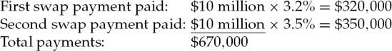
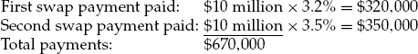
First, let's look at the payments that must be made by the asset manager. The first swap payment made by the asset manager is 3.2% (4.8% plus 160 bps divided by two) multiplied by the $10 million notional amount. The second swap payment made is 3.5% (5.4% plus 160 bps divided by two) multiplied by the $10 million notional amount. Thus,
The payments that will be received by the asset manager are the two coupon payments plus the change in the value of the reference asset. There will be two coupon payments. Since the coupon rate is 9% the amount received for the coupon payments is $900,000.
Finally, the change in the value of the reference asset must be determined. At the end of one year, the reference asset has a maturity of 9 years. Since the 9-year Treasury rate is assumed to be 7.6% and the credit spread is assumed to decline from 280 bps to 180 bps, the reference asset will sell to yield 9.4%. The price of a 9%, 9-year bond selling to yield 9.4% is 97.61. Since the par value is $10 million, the price is $9,761,000. The capital loss is therefore $239,000. The payment to the total return receiver is then:
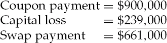
Netting the swap payment made and the swap payment received, the asset manager must make a payment of $9,000 ($661,000 - $670,000).
Notice that even though the asset manager's expectations were realized (that is, a decline in the credit spread), the asset manager had to make a net outlay. This illustration highlights one of the disadvantages of a total return swap noted earlier: The return to the investor is dependent on both credit risk (declining or increasing credit spreads) and market risk (declining or increasing market rates). Two types of market interest rate risk can affect the price of a fixed income asset. Credit-independent market risk is the risk that the general level of interest rates will change over the term of the swap. This type of risk has nothing to do with, the credit deterioration of the reference asset. Credit-dependent market interest rate risk is the risk that the discount rate applied to the value of an asset will change based on either perceived or actual default risk.
In the illustration, the reference asset was adversely affected by market interest rate risk, but positively rewarded for accepting credit dependent market interest rate risk. To remedy this problem, a total return receiver can customize the total return swap transaction. For example, the asset manager could negotiate to receive the coupon income on the reference asset plus any change in value due to changes in the credit spread. Now the asset manager has expressed a view exclusively on credit risk; credit independent market risk does not affect the swap value. In this case, in addition to the coupon income, the asset manager would receive the difference between the present value of the reference asset at a current spread of 280 bps and the present value of the reference asset at a credit spread of 180 bps.
An asset manager typically uses a credit default swap to hedge a credit exposure. However, a total return swap is typically used to increase credit exposure. A total return swap transfers all of the economic exposure of a reference asset to the total return receiver. In exchange for accepting this exposure, the total return receiver pays a floating interest rate to the total return payer.
Total return swap applications fall into three categories:
Asset managers using a total return swap for leveraging purposes.
Asset managers using a total return swap as a more transactionally efficient means for implementing a portfolio management strategy.
Managers of bank portfolios using a total return swap as an efficient vehicle for transferring credit risk and as a means for reducing capital charges.
Below, we provide two applications of total return swaps and further when total return index swaps are discussed.
There are a number of reasons why asset managers may wish to enter into total swap arrangements. As noted above, one of these is to reduce or remove credit risk. Using total return swaps as a credit derivative instrument, a party can remove exposure to an asset without having to sell it. In a vanilla total return swap the total return payer retains rights to the reference asset, although in some cases servicing and voting rights may be transferred. This assumes that the reference asset is on the payer's balance sheet.
The total return receiver gains an exposure to the reference asset without having to pay out the cash proceeds that would be required to purchase it. As the maturity of the swap rarely matches that of the reference asset, in a positive yield curve environment the swap receiver may gain from the positive funding or carry that derives from being able to roll over short-term funding of a longer-term asset. The total return payer on the other hand benefits from protection against interest rate and credit risk for a specified period of time, without having to liquidate the asset itself. At the maturity of the swap the total return payer may reinvest the asset if it continues to own it, or it may sell the asset in the open market. In this respect a total return swap is in essence a synthetic repo.
A total return swap agreement entered into as a credit derivative is a means by which banks can take on unfunded off-balance sheet credit exposure. Higher-rated banks that have access to London Interbank Bid Rate (LIBID) funding can benefit by funding on-balance-sheet assets that are credit protected through a credit derivative such as a total return swap, assuming the net spread of asset income over credit protection premium is positive.
A total return swap conducted as a synthetic repo is usually undertaken to effect the temporary removal of assets from the balance sheet. This may be desired for a number of reasons, for example if the institution is due to be analyzed by credit rating agencies, or if the annual external audit is due shortly. Another reason a bank may wish to temporarily remove lower-credit-quality assets from its balance sheet is if it is in danger of breaching capital limits in between the quarterly return periods. In this case, as the return period approaches, lower quality assets may be removed from the balance sheet by means of a total return swap, which is set to mature after the return period has passed.
However, this is a semantic point associated with the motivation of the total return payer. If effected for regulatory capital reasons a total return swap is akin to a synthetic repo; if effected for credit speculation reasons it becomes a credit derivative.
Let's use an actual case to see how a total return swap can be employed in the bank loan market (This illustration is an expanded discussion of a bank loan swap presented by Keith Barnish, Steve Miller, and Michael Rushmore [1997].) Consider the details of a 3-year swap on a term bank loan. A large AA insurance company purchased a 3-year total return swap on a $10 million piece of Riverwood International's Term Loan B. Term Loan B was actually a tranche of $250 million, but the insurance company only wanted credit exposure to a portion of the term loan.
This demonstrates one of the advantages of a credit derivative in general: customization. An investor may like the credit risk of a particular bank loan tranche, but may not have sufficient appetite for the whole loan. A total return credit swap allows the investor to choose a big or small piece of credit exposure depending on the investor's appetite for the credit risk. Furthermore, the term loan had a maturity of 10 years, while the holding period horizon of the insurance company was three years. Therefore, the total return swap can accommodate the insurance company's investment horizon while the term loan does not.
The seller of the swap (that is, the total return payer) was a large institutional bank. In order for the insurance company to purchase the total return swap, the bank effectively loaned the insurance company the $10 million notional amount of the swap. The bank in fact did not disburse $10 million to the insurance company, but instead charged the insurance company interest on $10 million dollars as if the bank had loaned the full amount. In this transaction, the bank charged the insurance company LIBOR + 75 bps. Since the insurance company's normal borrowing rate was 12.5 bps over LIBOR, the bank effectively charged the insurance company a swap processing fee of 62.5 bps, equivalent to $62,500 on an annual basis. In addition to the annual fee, the insurance company was required to put up $1 million of collateral as security for the effective loan. This $1 million was invested in U.S. Treasury securities.
In return for paying this fee, the insurance company received the total return on the Riverwood International term loan. The total return included the floating interest on the term loan of LIBOR + 300 bps plus any gain or loss in market value of the loan. In sum, the bank passed through the swap to the insurance company all of the interest payments and price risk as if the insurance company had the term loan on the asset side of its balance sheet.
The benefit to the insurance company was the net interest income earned on the swap. The insurance company agreed to pay LIBOR + 75 bps to the bank in return for LIBOR + 300 bps received from the Riverwood International term loan. The annual net interest income from the swap paid to the insurance company was:
Provided that Riverwood International did not default on any portion of the term loan, the insurance company also received the interest income on the Treasury securities.
Why would the bank want to enter into this transaction? Perhaps, the bank bit off more than it wanted to chew when it purchased the full tranche from Riverwood International. The total return swap with the insurance company allowed the bank to reduce its credit exposure and collect a fee. In effect, the bank got paid to reduce its credit risk.
And what about the insurance company? Was this a good deal for it? The answer is yes if we consider the alternative to the total return swap. Assume, that instead of the total return swap, the insurance company could have purchased a $10 million portion of the Riverwood International term loan at its normal financing cost of LIBOR + 12.5 bps, held the term loan on its balance sheet for three years, and then sold it at the end of its holding period. The question we need to answer is which alternative provided a greater return: the total return swap or the outright purchase of the term loan?
Table 43.1 details the holding period returns to the two alternatives. In the first case, the insurance company borrows $1 million at its normal financing rate to purchase the Treasury security collateral and receives three annual net payments of $225,000 from the bank as well as interest income on the Treasury securities. Additionally, in year 3, the insurance company receives back the $1 million of collateral. These cash flows are discounted at the insurance company's cost of capital of 3-year LIBOR + 12.5 bps.
In the second case, the insurance company receives the full payment of LIBOR + 300 bps on the term loan, but must finance the full $10 million for three years. It receives an annual cash flow of $950,000, and sells its investment at the end of three years for $10 million.
To keep the analysis simple, assume that the insurance company bought a 3-year U.S. Treasury note as collateral with a maturity equal to the tenor of the swap and with an annual coupon of 6.00%, that 1-year LIBOR remains constant at 5.78125%, and that there is no change in value of the Riverwood International term loan. The discount rate for present value purposes is 5.90625% (LIBOR + 12.5 bps).
Under the swap, the insurance company will receive each year a cash flow of $225,000 from the bank and $60,000 from the Treasury note. In addition, in year 3, the insurance company will receive back its $1 million collateral contribution. Under the outright purchase of the term loan, the insurance company will receive each year a cash flow of $950,000. At the end of three years the insurance company sells the term loan in the market for its original investment of $10 million. Table 43.1 details these assumptions as well as a comparison of the cash flows for each alternative.
As can be seen from Table 43.1, the outright purchase of the term loan results in a higher net present value than the total return swap. The net present value for the term loan is $961,833 and for the total return swap it is $604,983, a difference of $356,850. However, the total return swap requires a much smaller capital requirement than the outright purchase of the term loan. Even though the total return swap results in lower total cash flows, it provides an internal rate of return (IRR) that is three times greater than that of the term loan purchase.
This example demonstrates the use of leverage in a total return swap. The smaller capital commitment of the total return swap allows the insurance company to earn a higher rate of return on its investment than the outright purchase of the term loan. In fact, the leverage implicit in this total return swap is 10:1. Economically, the total return swap is more efficient because it allows the insurance company to access the returns of the bank loan market with a smaller required investment.
However, what if the value of the term loan had declined at the end of three years? Assume that over the 3-year holding period, the value of the Riverwood International bank loan declined in value to $9 million. With the total return swap arrangement, the $1 million loss in value would wipe out the posted collateral value. At the end of year 3, the insurance company would receive only the cash flow from the interest income, $225,000 from the swap, and $60,000 in interest from the posted collateral.
Under the purchase scenario, the insurance company would receive back $9 million of its committed capital. Additionally, in each year the insurance company would receive the $950,000 interest income from the term loan. Table 43.1 also compares the two investment choices under the assumption of a $1 million decline in loan value.
Under the total return swap, the net present value of the investment is now a negative $236,868. Conversely, a decline in loan value of $1 million still leaves the purchase scenario with a positive net present value of $120,431. Comparing the IRR on the two investments, we now see that the total return swap yields a negative IRR of —7%, while the purchase of the term loan yields a positive IRR of 6%—slightly more than the insurance company's cost of borrowed funds. Table 43.1 demonstrates that the embedded leverage in the total return swap can be a double-edged sword. It can lead to large returns on capital, but can also result in rapid losses.
Thus far our focus has been on a single reference asset. Total return index swaps are swaps where the reference asset is the return on a market index. The market index can be an equity index or a bond index. Our focus will be on bond indices.
Broad-based bond market indices such as the Lehman, Salomon Smith Barney, and Merrill Lynch indexes have subindexes that represent major sectors of the bond market. For example there is the Treasury and agency sector, the credit sector (that is, investment-trade corporate bonds, at one time referred to as the corporate sector), the mortgage sector (consisting of agency residential mortgage-backed securities), the commercial mortgage-backed securities (CMBS) sector, and the asset-backed securities (ABS) sector. The non-Treasury sectors offer a spread to Treasuries and are hence referred to as "spread sectors." The spread in the mortgage sector is primarily compensation for the prepayment risk associated with investing in this sector. Spread to compensate for credit risk is offered in the credit spread sector, of course, and the CMBS and ABS sectors. There are also indexes available for other credit spread sectors of the bond market: high-yield corporate bond sector and emerging market bond sector. Thus, a total return index swap in which the underlying index is a credit spread sector allows an asset manager to gain or reduce exposure to that sector.
Below, we discuss the flexibility offered asset managers and hedge fund managers by using total return swaps in which the index is a credit spread sector of the bond market.
Bond portfolio strategies range from indexing to aggressive active strategies. The degree of active management can be quantified in terms of how much an asset manager deviates from the primary risk factors of the target index. A bond indexing strategy for a sector involves creating a portfolio so as to replicate the issues comprising the target sector's index. This means that the indexed portfolio is a mirror image of the target sector index or, put another way, that the ex ante tracking error is close to zero.
Why would an asset manager pursuing an active portfolio management strategy want to engage in an indexing strategy for a credit sector of the target index? Suppose that the asset manager's target index is the Lehman Brothers U.S. Aggregate Bond Index. Suppose further that the asset manager skills are such that she believes she can add value in the mortgage, CMBS, and ABS sectors but has no comparative advantage in the credit (corporate sector). The asset manager in this case can underweight the credit sector. However, the risk is that the credit sector will perform better than the other sectors in the target index and, as a result, the asset manager will underperform the target index. An alternative is to be neutral with respect to the credit sector and make active bets within the sectors of the target index that the asset manager believes value can be added. This approach requires that the asset manager follow an indexing strategy for the credit sector of the target index. However, in pursuing this strategy of creating a portfolio to replicate the credit sector, the asset manager will encounter several logistical problems.
First, the prices for each issue in the credit sector used by the organization that publishes the sector index may not be execution prices available to the asset manager. In fact, they may be materially different from the prices offered by some dealers. In addition, the prices used by organizations reporting the value of sector indexes are based on bid prices. Dealer ask prices, however, are the ones that the manager would have to transact at when constructing or rebalancing the indexed portfolio. Thus there will be a bias between the performance of the sector index and a portfolio that attempts to replicate the sector index that is equal to the bid-ask spread.
Furthermore, there are logistical problems unique to certain sectors in the bond market. For the credit sector, which consists of investment-grade corporate bonds, there are typically more than 4,000 issues. Because of the illiquidity for many of the issues, not only may the prices used by the organization that publishes the index be unreliable, but also many of the issues may not even be available.
Third, as bonds mature, their shrinking duration will force them out of this index. This will create natural turnover and higher transaction costs. Last, bonds pay consistent coupons that must be reinvested in the index.
In the absence of a total return swap, there are two methodologies that have been used to construct a portfolio to replicate the index representing the credit sector: stratified sampling methodology and the variance minimization methodology. With the stratified sampling approach (or also called the cellular approach) to indexing, the sector index is divided into cells representing the primary risk factors. The objective is then to select from all of the issues in the index one or more issues in each cell that can be used to represent that entire cell. The total dollar amount purchased of the issues from each cell will be based on the percentage of the index's total market value that the cell represents. For example, if X% of the market value of all the issues in the credit sector index is made up of single-A-rated corporate bonds, then X% of the market value of the replicating portfolio should be composed of single-A-rated corporate bond issues. The number of cells that the asset manager uses will depend on the dollar amount of the portfolio to be indexed. In indexing a portfolio of less than $50 million, for example, using a large number of cells would require purchasing odd lots of issues. This increases the cost of buying the issues to represent a cell, and thus would increase the ex ante tracking error. Reducing the number of cells to overcome this problem increases ex ante tracking error because the major risk factors of the indexed portfolio may differ materially from those of the index. For corporate bonds, for example, there is the concern of downgrade risk of individual corporate issues that would adversely affect tracking error. Figure 43.2 shows the findings of a Lehman Brothers study that demonstrates how many issues must be purchased to minimize tracking error due to downgrade risk (see Dynkin, Hyman, and Konstantinovsky, 2002). As can be seen, if only a few issues are selected tracking error is high.
The variance minimization methodology is a more complicated approach than stratified sampling. This approach requires using historical data to estimate the variance of the tracking error for each issue in the index. The objective then is to minimize the variance of the tracking error in constructing the replicating portfolio.
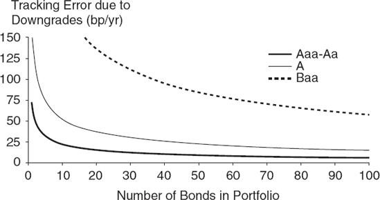
Figure 43.2. Risk due to Downgrades as a Function of Portfolio Size—by Credit Quality Source: Exhibit 14 in Dynkin, Hyman, and Konstantinovsky (2002), p. 100. This copyrighted material is reprinted with permission from Institutional Investor, Inc., Journal of Portfolio Management, 225 Park Avenue South, New York, NY 10003.
The more efficient solution may be simply to use an total return index swap where the credit sector to be indexed is the underlying index for the swap.
Active bond portfolio strategies involve constructing a portfolio that deviates from the target index. There are various strategies that can be employed. For example, one strategy is to construct a portfolio that is intentionally different from the duration of the target index based on the view of the asset manager regarding future interest rates. Another is to overweight a sector of the index based on the asset manager's view of the relative performance of the sectors comprising the index. For example, if the credit sector is expected to outperform the other sectors, an asset manager may wish to overweight that sector. The asset manager can monetize this view by entering into a total return swap as the total return receiver. Again, as noted earlier, this is an efficient way to replicate the performance of the index.
Hedge funds manager can use total return swaps to create leverage in the same way described earlier when we showed how a synthetic repo can be created for a credit-risky bond. Moreover, suppose instead that a hedge fund manager believes that the credit sector will have a negative return. The manager can monetize this view by selling a total return swap. The advantage of the total return swap is that the credit sector can be shorted, a task that is extremely difficult and costly to do for individual bond issues in the credit sector.
Total return swaps can be sued as effective risk control instruments. Interest rate swaps can be used to control the duration of the portfolio. Total return swaps can be used to control the spread duration of a portfolio and, more specifically, the credit spread duration of a portfolio, that is the sensitivity of a portfolio to changes in credit spreads. Hedging a position with respect to credit spread risk means creating a cash and total return swap position whereby the credit spread duration is zero. An asset manager would want to hedge a portfolio that has exposure to credit spread risk if the credit spread duration of the portfolio differs from that of the target index. Total return swaps can be used to bring the portfolio's credit spread risk duration in line with the credit spread risk of the target index.
In a total return swap, the total return receiver (or swap buyer) agrees to make to floating-rate payments on designated dates to the total return payer (or swap seller) in exchange for the total return realized on a reference asset. In the fixed income market, the reference asset can be a credit-risky bond, a reference portfolio, or an index representing a sector of the bond market. Total return swaps can be used by fixed income managers for leveraging purposes or to more efficiently implement a portfolio strategy. In addition, total return swaps are an efficient vehicle for allowing bank portfolio managers to transfer credit risk and thereby reduce capital charges. Total return index swaps can be used for a wide range of bond portfolio strategies, ranging from indexing to aggressive active strategies.
Anson, M. J. P., Fabozzi, F. J., Choudhry, M., and Chen, R-R (2004). Credit Derivatives: Instruments, Pricing, and Applications. Hoboken, NJ: John Wiley & Sons.
Barnish, K., Miller, S., and Rushmore, M. (1997). The new leveraged loan syndication market. Journal of Applied Corporate Finance (Spring): 79-88.
Dynkin, L., Hyman, J., and Konstantinovsky, V. (2002). Sufficient diversification in credit portfolios. Journal of Portfolio Management (Fall): 89-114.
Goodman, L. S., and Fabozzi, F. J. (2005). CMBS total return swaps. Journal of Portfolio Management, Special Issue on Real Estate: 162-167.
Kolb, R. and Overdahl, J. (2007). Futures, Options and Swaps. Oxford: Blackwell.