Sorting and Filtering a PivotTable

To make a PivotTable show the data you require, you may need to sort it or filter it.

To sort a PivotTable, click the pop-up button of the field by which you want to sort. Excel displays the sorting and filtering window for that field. The window bears the field's name, as you can see in Figure 12–19, which shows the sorting and filtering window for the Product field. You can then click the Ascending button to produce an ascending sort (from A to Z, from small numbers to large numbers, and from early dates and times to later ones) or the Descending button to produce a descending sort (the opposite).

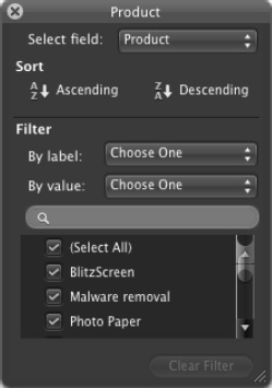
Figure 12–19. To sort or filter a PivotTable, open the sorting and filtering window for the field, then choose options in the Sort area or the Filter area. The sorting and filtering window's title bar shows the field's name (here, Product).

When you apply sorting to a field, the field name pop-up button changes to show an arrow indicating the direction of the sort. For example, in Figure 12–20, you can see an upward arrow indicating a descending sort on the Salesperson field and a downward arrow indicating an ascending sort on the Product field. The Line field shows the regular pop-up button.

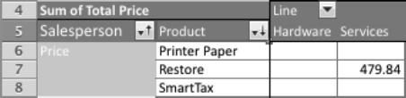
Figure 12–20. When you sort a PivotTable, the field's pop-up button shows an upward arrow for a descending an sort (as on the Salesperson field here) or a downward arrow for ascending sort (as on the Product field here).

To filter the PivotTable, click the pop-up button next to the field's name to display the sorting and filtering window, then choose the filtering criteria in the Filter area. Here are some examples:

• Filter by label. To filter by label, open the By label pop-up menu, choose the comparison type, then specify the data required. For example, choose the Contains comparison to find labels that match the text string you type in the text box that appears, as shown on the left in Figure 12–21.

Figure 12–21. You can filter a field by its label (as shown on the left here) or by its value. You can also search in the Search box or clear the check boxes of items you want to exclude.

• Filter by value. To filter by value, open the By value pop-up menu,then choose the comparison you want. For example, choose the Top 10 item to create a top-however-many-you-choose filter, then set the number of items in the left of the two pop-up menus that appear below the By value pop-up menu when it's showing Top 10 (see the right screen in Figure 12–21). In the right of the two pop-up menus, choose Item, Percentage, or Sum as needed for the filtering.
• Filter by individual values. To filter by individual values, clear the (Select All) check box in the lower part of the Filter area, then select the check box for each item you want to use in the filter. To find only particular items so that you can select or clear their check boxes, click in the Search box,then type the search term.

When you apply a filter, the field's pop-up button displays a funnel-like filter symbol, as you can see on the Line field in Figure 12–22.

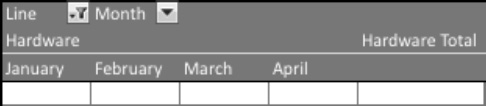
Figure 12–22. Excel displays a funnel-like filter on a field's pop-up button to indicate that you've applied filtering to that field.

To remove filtering, open the sorting and filtering window again, then click the Clear Filter button at the bottom.