
Navigating Quickly Through Worksheets and Workbooks
To work swiftly and easily in Excel, you need to know the best ways of navigating through worksheets and workbooks. We'll look at these in this section—after we check that we're using the same terms to refer to the elements in the Excel user interface.
Elements of the Excel User Interface
When you've created a new workbook or opened an existing one, Excel displays the workbook's worksheets. Figure 1–10 shows Excel with a workbook open and the main elements of the user interface labeled.
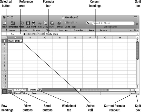
Figure 1–10. The main elements of the Excel application window and a workbook
- Formula bar. This is the bar below the Ribbon. This area shows the data or formula in the active cell and gives you an easy place to enter and edit data.
- Reference area. This area appears at the left end of the formula bar. It shows the active cell's address (for example, A1) or the name you've given the cell so as to refer to it easily.
- Row headings. These are the numbers at the left side of the screen that identify each row. The first row is 1, the second row 2, and so on, up to the last row, 1048576.
- Column headings. These are the letters at the top of the worksheet grid that identify the columns.
- The first column is A, the second column B, and so on up to Z.
- Excel then uses two letters: AA to AZ, BA to BZ, and so forth until ZZ.
- After that, Excel uses three letters: AAA, AAB, and so on up to the last column, XFD.
- Cells. These are the boxes formed by the intersections of the rows and columns. Each cell is identified by its column letter and row number. For example, the first cell in column A is cell A1 and the second cell in column B is cell B2. The last cell in the worksheet is XFD1048576.
- Active cell. This is the cell you're working in—the cell that receives the input from the keyboard. Excel displays a blue rectangle around the active cell.
- Select All button. Click this button at the intersection of the row headings and column headings to select all the cells in the worksheet.
- Worksheet tabs. Each worksheet has a tab at the bottom that bears its name. To display a worksheet, you click its tab in the worksheet tabs area.
- Scroll buttons. Click these buttons to scroll the worksheet tabs so you can see the ones you need. Click the leftmost button to scroll all the way back to the first tab, or click the rightmost button to scroll to the last tab. Click the two middle buttons to scroll back or forward by one tab.
- View buttons. Click these buttons to switch between Normal view and Page Layout view. You'll learn how to use these views later in this chapter.
- Split boxes. You use these boxes when you need to split the worksheet window into two or four areas. You'll learn how to do this in the section “Splitting the Window to View Separate Parts of a Worksheet” later in this chapter.
- Current formula readout. This readout shows you the result of any of six common formulas—AVERAGE, COUNT, COUNTNUMS, MIN, MAX, or SUM—as applied to the current cell or range. You can click the readout to switch formulas, or choose the None item to display no formula result. For example, if you select cells B1:B4 and choose the SUM formula, you'll see the total produced by the values in these cells.
Navigating Among Worksheets
Each workbook consists of one or more worksheets or other sheets, such as chart sheets or macro sheets. You can use as many worksheets as you need to separate your data conveniently within a single workbook file. For example, you can have a separate budget-planning worksheet for each department in a single workbook file rather than having a separate workbook for each department.
To display the worksheet you want to use, click its tab in the worksheet tab bar (see Figure 1–11). If the worksheet's tab isn't visible in the worksheet tab bar, click the scroll buttons to display it (unless you've hidden the worksheet).
TIP: If you want to make the worksheet tab bar wider so you can see more tabs at once, drag the divider bar to the right. Excel makes the horizontal scroll bar smaller to compensate.
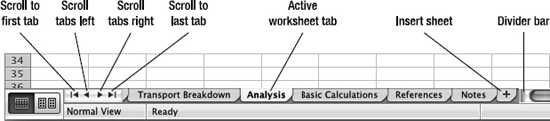
Figure 1–11. Use the worksheet tab bar to display the worksheet you want or to insert a new worksheet. You can drag the divider bar to change the length of the tab bar.
TIP:1You can quickly move to the next worksheet by pressing Cmd+Page Down or to the previous worksheet by pressing Cmd+Page Up.
Changing the Active Cell
In Excel, you usually work in a single cell at a time. That cell is called the active cell and it receives the input from the keyboard.
You can move the active cell easily using either the mouse or the keyboard:
- Mouse. Click the cell you want to make active.
- Keyboard. Press the arrow keys to move the active cell up or down by one row or left or right by one column at a time. You can also press the keyboard shortcuts shown in Table 1-1 to move the active cell further.
TIP: If your Mac's keyboard doesn't have the Home key, End key, Page Up key, and Page Down key, you'll need to use function-key shortcuts. Press Fn+left arrow for Home, Fn+right arrow for End, Fn+up arrow for PageUp, and Fn+down arrow for PageDown. Use these keys as needed with the keyboard shortcuts in Table 1–1—for example, press Cmd+Fn+left arrow to move to the first cell in the active worksheet.
Table 1–1. Keyboard Shortcuts for Changing the Active Cell
| To Change the Active Cell | Press This Keyboard Shortcut |
| To the first cell in the row | Home |
| To the first cell in the active worksheet | Cmd+Home |
| To the last cell used in the worksheet | Cmd+End |
| Down one screen | Page Down |
| Up one screen | Page Up |
| Right one screen | Option+Page Down |
| Left one screen | Option+Page Up |
| To the last row in the worksheet | Cmd+down arrow |
| To the last column in the worksheet | Cmd+right arrow |
| To the first row in the worksheet | Cmd+up arrow |
| To the first column in the worksheet | Cmd+left arrow or Home |
| To the next corner cell clockwise in a selected range | Ctrl+. (Ctrl and the period key) |
Selecting and Manipulating Cells
To work with a single cell, you need only click it or use the keyboard to make it the active cell. When you need to affect multiple cells at once, you select the cells using the mouse or keyboard.
Excel calls a selection of cells a range. A range can consist of either a rectangle of contiguous cells or two or more cells that aren't next to each other. The left illustration in Figure 1–12 shows a range of contiguous cells, while the right illustration shows a range of separate cells.
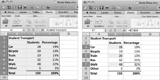
Figure 1–12. You can select either a range of contiguous cells (left) or a range of individual cells (right). Excel darkens the headers of the rows and columns that contain the range to make the range easier to see.
You can select a range of contiguous cells in any of these three ways:
- Click and drag. Click the first cell in the range, then drag to select all the others. For example, if you click cell B2 and then drag to cell E7, you select a range that's four columns wide and six rows deep. Excel uses the notation B2:E7 to describe this range—the starting cell address, a colon, and then the ending cell address.
- Click and then Shift+click. Click the first cell in the range, then Shift+click the last cell. Excel selects all the cells in between. You can use this technique anytime, but it's most useful when the first cell and last cell are widely separated; for example, when the first cell and last cell don't appear in the Excel window at the same time.
- Hold down Shift and use the arrow keys. Use the arrow keys to move the active cell to where you want to start the range; then hold down Shift and use the arrow keys to extend the selection for the rest of the range. This method is good if you prefer using the keyboard to the mouse.
You can select a range of noncontiguous cells by clicking the first cell (or dragging through a range of contiguous cells) and then holding down Cmd while you click other individual cells or drag through ranges of contiguous cells. Excel uses commas to separate the individual cells in this type of range. For example, the range D3,E5,F7,G1:G13 consists of three individual cells (D3, E5, and F7) and one range of contiguous cells (G1 through G13).
NOTE: You can quickly select a row by clicking its row heading or pressing Shift+spacebar when the active cell is in that row. Likewise, you can select a column by clicking its column heading or pressing Ctrl+spacebar. To select all the cells in the active worksheet, click the Select All button (where the row headings and column headings meet). You can also either press Cmd+A or press Shift+spacebar followed by Ctrl+spacebar (or vice versa).
To deselect a range you've selected, click anywhere outside the range.