Tools for Entering Text and Formulas Quickly

The most straightforward way of entering text and formulas in your workbooks is to type it in. But no matter how fast you type, it pays to know all the alternative ways of getting data and formulas into your workbooks. These range from importing the data from an existing file, connecting to an external data source, speeding up data entry by maxing out AutoCorrect, taking advantage of the powerful AutoFill feature, and using copy and paste in all its flavors. You can even using the Replace feature to enter text.

Importing Data

If you have the data you need in an existing file, you can usually import it into Excel. Excel can import files in these five formats:

• Comma-separated values (CSV). A CSV file uses a comma to separate the contents of cells.
• Tab-separated values (TSV). A TSV file uses a tab to separate the contents of cells.

• Space-separated values. A space-separated values file (not usually referred to as SSV) uses a space to separate the contents of cells.
• FileMaker Pro database. FileMaker Pro is a heavy-duty database application that runs on both Mac OS X and Windows. FileMaker Pro files use the .fp7 file extension.
• HTML. HTML (HyperText Markup Language) is the markup language used for Web pages.

To import data from an existing file, follow these steps:

1. Open the workbook you want to import the data into. If you want to put the data in a new workbook, press Cmd+N to create one.
2. Choose File Import to display the Import dialog box (see Figure 1–13).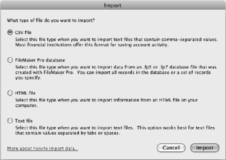
   

   Figure 1–13. In the Import dialog box, select the appropriate option button based on the type of file you want to import.

3. Select the CSV file option button, the FileMaker Pro database option button, the HTML file option button, or the Text File option button (for tab-separated files or space-separated files).

   NOTE: To import data from a FileMaker Pro database, you must have FileMaker Pro installed on your Mac. Without FileMaker Pro, Excel can't read a FileMaker Pro database.

4. Click the Import button to display the dialog box for identifying the file. The name of this dialog box varies depending on your choice in step 3: it's the Choose a File dialog box for CSV files or text files, the Choose a Database dialog box for FileMaker Pro, and the Open: Microsoft Excel dialog box for HTML files.
5. Choose the file that contains the data and then click the Get Data button, the Choose button, or the Open button (depending on the dialog box).
6. Follow the steps of the Import Wizard that opens. The following sections explain the main considerations.

Importing Data from a Comma-Separated Values File or a Text File

When you import data from a comma-separated values file or a text file, the Text Import Wizard walks you through the import process.

On the wizard's first screen (see Figure 1–14), start by making sure that Excel has selected the Delimited option button if your file is delimited with commas, tabs, or another character. If it's a text file that uses spaces to create fixed-width columns, select the Fixed width option button.

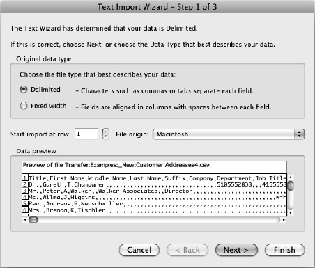
Figure 1–14. Make sure that the Text Import Wizard has made the right choice between the Delimited option button and the Fixed width option button. You can also decide at which row to start importing.

If you need to skip some rows at the beginning of the file, increase the value in the Start import at row box. To start from the beginning, make sure this box is set to 1.

If the preview in the Data preview box looks wrong, open the File origin pop-up menu, and choose the encoding the file uses. For example, if the file was created on a Windows PC, you may need to choose the Windows (ANSI) item to make the text display correctly. If the file was created on a Mac, choosing Macintosh in the File origin pop-up menu should do the trick.

When the preview looks okay, click the Next button to move to the second screen (see Figure 1–15).

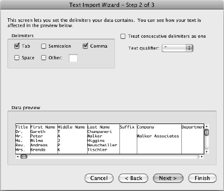
Figure 1–15. On the second screen of the Text Import Wizard for a CSV or TSV file, make sure that Excel has identified the correct delimiters.

In the Delimiters box, make sure Excel has selected the check box for the delimiter the file uses—for example, the Tab check box.

Select the Treat consecutive delimiters as one check box if you want Excel to treat two or more consecutive delimiters as a single delimiter. Using this setting has the effect of collapsing blank fields in the data. Normally, you won't need to use this setting.

If your data file uses single quotes or double quotes to mark strings of text, make sure that Excel has selected the right type of quotes in the Text qualifier pop-up menu. If not, select it yourself.

Check that the data in the Data preview box looks okay, and then click the Next button to display the third and final screen of the Text Import Wizard (see Figure 1–16). On this screen, you can set the data format of any column by clicking the column in the Data preview box and then selecting the appropriate option button in the Column data format box:

• General. The Text Import Wizard suggests this format for most columns. The General format makes Excel convert numeric values to numbers, convert date values to dates, and treat any other type of data as text. This works pretty well for most fields, so you may want to simply leave this setting. Otherwise, you can set each field to the type needed.
• Text. Select this format for any data you want Excel to treat as text. Sometimes you may want to set this format for data that Excel would otherwise convert to numbers.
• Date. Select this format to make sure Excel knows that a column contains dates. In the pop-up menu, choose the order in which the month (M), day (D), and year (Y) appear: MDY, DMY, YMD, MYD, DYM, or YDM. If you're using the U.S. localization, Excel uses the MDY format by default so you won't need to change it unless the file has come from somewhere that treats dates differently.
• Do not import column (Skip). Select this button for any column you want to skip. This option can be great for data you're sure you don't need, though you may find it easier to import all of the columns and delete those you don't need after the import.

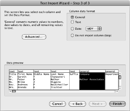
Figure 1–16. On the third screen of the Text Import Wizard for a CSV or TSV file, you can set the data format for each column. You can also tell Excel not to import particular columns you don't need.

When you finish choosing text-import settings, click the Finish button. The Text Import Wizard imports the data into the active worksheet.

Importing Data from a FileMaker Pro Database

When you import data from a FileMaker Pro database, the FileMaker Pro Import Wizard (see Figure 1–17) walks you through the process of choosing the right fields.

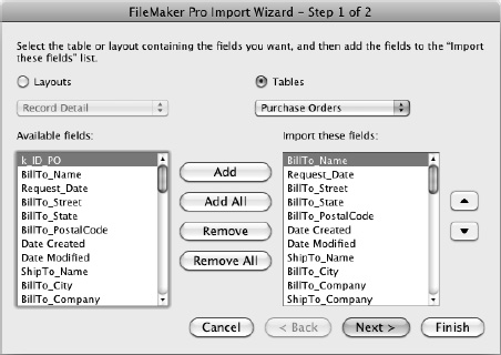
Figure 1–17. On the first screen of the FileMaker Pro Import Wizard, choose the layout or table you want to import, pick the fields, and then arrange them into your preferred order.

On the first screen of the FileMaker Pro Import Wizard, follow these steps:

1. Click the Layouts option button if you want to use a layout. Click the Tables option button if you want to use a table.
2. Open the pop-up menu below the Layouts option button or Tables option button (whichever you chose), and then click the layout or table you want to use. Excel displays the fields from the layout or table in the Available fields list box.
3. Add the fields you need to the Import these fields list box:
   • Add a single field. Click the field in the Available fields list box and then click the Add button. Repeat as needed.
   • Add all the fields. Click the Add All button. Often, you'll want to add all the fields and then remove a few of them.
   • Remove a field. Click the field in the Import these fields list box and then click the Remove button.
   • Remove all fields. Click the Remove All button.
4. In the Import these fields list box, put the fields in your preferred order. To move a field up or down, click it and then click the Move Up button (the button with the up arrow) or the Move Down button (the button with the down arrow).

When you've chosen the fields you want and arranged them into your preferred order, click the Next button to display the second and final screen of the FileMaker Pro Import Wizard (see Figure 1–18). On this screen, you can set the criteria to pick only the records you want from the table or layout you chose.

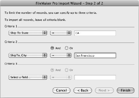
Figure 1–18. On the second screen of the FileMaker Pro Import Wizard, set up the criteria needed to limit the import to only the records you want.

If you want all the records in the table or layout, you can simply click the Finish button. But if you want to strip the table or layout down to only records that match particular criteria, follow these steps:

1. In the Criteria 1 area, set up your first criterion:
   • Open the left pop-up menu and click the field to use for the criterion.
   • Open the middle pop-up menu and click the comparison: =, <=, >=, <, >, begins with, ends with, or contains.
   • In the text box, specify the value for the comparison.
2. If you need a second criterion, select the appropriate option button:
   • Select the And option button to make the records match the first criterion and the second criterion—for example, Ship To State = CA and Ship To City = San Francisco.
   • Select the Or option button to make the records match either the first criterion or the second criterion—for example, Ship To State = CA or Ship To State = AZ.
3. Set up the second criterion in the Criterion 2 box using the same technique as for the first.
4. If you need a third criterion, select the And option button or the Or option button (as appropriate), and then use the third line of controls to specify the criterion.

When you've nailed down your criteria, click the Finish button to close the FileMaker Pro Import Wizard. The Wizard displays the Returning External Data to Microsoft Excel dialog box (see Figure 1–19).

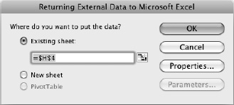
Figure 1–19. In this dialog box, choose the Existing sheet option button or the New sheet option button as appropriate. Then click the OK button.

In the Where do you want to put the data area, select the Existing sheet option button if you want to put the incoming data on the worksheet you've selected. Usually, this is the best bet. The text box shows the active cell; if you need to change it, you can type a different address, or click in the workbook and then click the cell you want to use as the upper-left corner of the range. Otherwise, if you want to create a new worksheet and put the data on it, select the New sheet option button.

Click the OK button to close the Returning External Data to Microsoft Excel dialog box. The Wizard queries the database, returns the records that match your criteria, and then enters them in the worksheet you specified.

Importing Data from an HTML File

When you import data from an HTML file, Excel simply opens the file without displaying any Import Wizard screens. You can then manipulate the contents of the file as needed.

Connecting a Worksheet to External Data Sources

If you have an external data source that contains data you need to use in your Excel worksheet, you can connect the worksheet to the data source and pull in the data so you can work with it in Excel.

To get the data into the worksheet, you use the same tools we just discussed for importing data—for example, you use the FileMaker Pro Import Wizard to import data from a FileMaker Pro database. After importing the data, you can refresh some or all of it as needed, updating the worksheet with the latest data from the data source.

Chapter 11 explains how to work with external data.

Entering Text Using AutoCorrect

As you work in a worksheet, the AutoCorrect feature analyzes the characters you type and springs into action if it detects a mistake it can fix or some formatting it can apply. This feature can save you a lot of time and effort and can substantially speed up your typing, so it's well worth using—but you need to set it up to meet your needs. AutoCorrect also has some features that can cause surprises, so you'll want to choose settings that suit the way you work.

Opening the AutoCorrect Preferences Pane

To set up AutoCorrect, choose Tools AutoCorrect from the menu bar to display the AutoCorrect preferences pane in the Excel Preferences dialog box (see Figure 1–20).

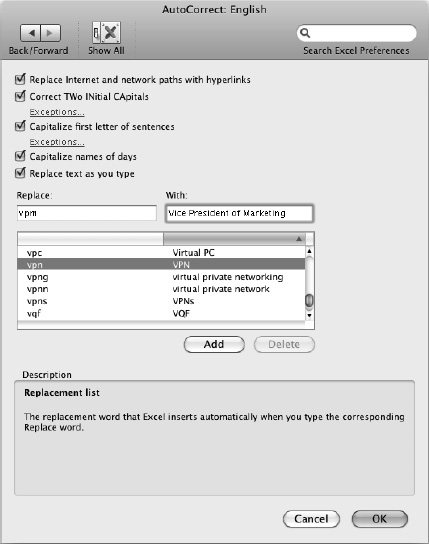
Figure 1–20. You can use AutoCorrect to enter text quickly in your worksheets as well as to correct typos and create hyperlinks.

Choosing Options to Make AutoCorrect Work Your Way

With the AutoCorrect preferences pane displayed, select the check box for each option you want to use:

• Replace Internet and network paths with hyperlinks. Select this check box to have AutoCorrect insert a hyperlink when you type a URL (for example, www.apress.com) or a network path (such as \server1users). This option is helpful if you want live hyperlinks in your workbooks—for example, if you're making a list of products with URLs, and you want to be able to click a link to open the web page in your browser.
• Correct TWo INitial CApitals. Select this check box to have AutoCorrect apply lowercase to a second initial capital—for example, changing “THree” to “Three.”
• Capitalize first letter of sentences. Select this check box if you want AutoCorrect to automatically start each new sentence in a cell with a capital letter. AutoCorrect doesn't capitalize the first sentence in the cell, as this option only kicks in once you've typed some text followed by a period. Clear this check box if you want to control capitalization yourself.
• Capitalize names of days. Select this check box to have AutoCorrect automatically capitalize the first letter of the day names (for example, Sunday). This option is usually helpful unless you're writing minimalist poetry in Excel.
• Replace text as you type. Select this check box to use AutoCorrect's main feature, replacing misspellings and abbreviations with their designated replacement text. You will want to use this feature to make the most of AutoCorrect.

Creating AutoCorrect Exceptions

If you select the Correct TWo INitial CApitals check box or the Capitalize first letter of sentences check box, you can create exceptions that tell AutoCorrect not to fix particular instances of two initial capitals or sentences.

To create exceptions, click the Exceptions link under either the Correct TWo INitial CApitals check box or the Capitalize first letter of sentences check box. Excel displays the AutoCorrect Exceptions dialog box; the left screen in Figure 1–21 shows the First Letter tab, and the right screen in Figure 1–21 shows the INitial CAps tab.

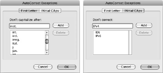
Figure 1–21. Use the First Letter tab and INitial CAps tab of the AutoCorrect Exceptions dialog box to set up exceptions to the rules for capitalizing the first letter of sentences or lowercasing the second letter of a word.

On the First Letter tab, list the terms that end with periods but after which you don't want the next word to start with a capital letter. Office starts you off with a list of built-in terms, such as vol. and wk. To add a term, type it in the Don't capitalize after text box, and then click the Add button.

On the INitial CAps tab, list the terms that start with two initial capital letters that you don't want AutoCorrect to reduce to a single capital—for example, IPv6. Type a term in the Don't correct text box, and then click the Add button to add it to the list.

On either tab, you can remove an existing term by clicking it in the list box, and then clicking the Delete button.

When you've finished setting up the exceptions, click the OK button to close the AutoCorrect Exceptions dialog box.

Creating Replace-As-You-Type Entries

Inserting missed capitals and creating hyperlinks automatically helps a bit, but the main point of AutoCorrect is to correct typing errors.

AutoCorrect comes with a list of standard errors, such as “abbout” for “about,” that you'll probably want it to correct automatically. But where you can really take advantage of AutoCorrect is by creating entries that aren't errors but rather abbreviations that you type deliberately and have AutoCorrect expand for you. For example, you can create an entry that changes “vpm” to “Vice President of Marketing” or one that changes “ssf” to “Second Storage Facility, Virginia (Security Grade II)”.

Creating AutoCorrect Entries

To create an AutoCorrect entry, follow these steps:

1. Type the entry name (the text that triggers the replacement) in the Replace box. The name can be up to 32 characters long, but shorter entries save you more time.

   TIP: When naming an AutoCorrect entry, you'll usually want to avoid using any words or names you may need to type in your workbooks. The exception is when you always want to change a particular word. For example, if your boss has a pet hate of the word “purchase,” you could set up AutoCorrect entries to change “purchase” to “buy,” “purchased” to “bought,” and so on.

2. Type or paste the replacement text in the With box. The replacement can be up to 255 characters long (including spaces and punctuation).

   NOTE: You can enter AutoCorrect entries only into a single cell. Even if you select multiple cells and paste them into the With box in the AutoCorrect pane, AutoCorrect strips out the cell divisions.

3. Click the Add button.

If you need to delete an existing entry, select it either by clicking in the Replace box and typing its name or by scrolling down to it and clicking it. Then click the Delete button.

Using Your AutoCorrect Entries

Once you've set up your AutoCorrect entries, Excel automatically replaces an entry after you type it and then press the spacebar or a punctuation key or move to another cell.

Entering Text with AutoFill and Custom Lists

In many workbooks, you'll need to enter a series of data, such as a list of months or years, a sequence of numbers, or a progression of dates (such as every Monday). In many cases, you can save time and effort by using Excel's AutoFill feature.

AutoFill works by analyzing the contents of one or more cells you select, and then entering the relevant series of data in the cells to which you extend the selection by dragging. AutoFill figures out mathematical sequences or date sequences on the fly and uses built-in custom lists to fill in the days of the week or the months of the year. You can also create your own custom lists for data you want to teach Excel to fill in.

Using AutoFill's Built-in Capabilities

The best way to grasp what you can do with AutoFill is to try it. So open a workbook you're comfortable experimenting with and try the examples in this section.

First, have AutoFill fill in the days of the week. Follow these steps:

1. Type Monday in cell A1 and click the Enter button on the Formula bar to enter the data. (If you prefer to press Return to enter the data, click cell A1 again to select it once more.)
2. Drag the AutoFill handle—the blue square that appears at the lower-right corner of the selection—down to cell A7. As you drag past each cell, AutoFill displays a ScreenTip showing the data it will fill in that cell (see Figure 1–22).
   

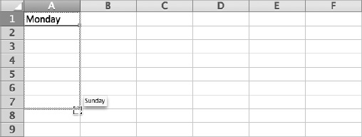
   Figure 1–22. Drag the AutoFill handle down or across to fill in a series of data derived from one or more existing entries. In this case, AutoFill fills in the days of the week and repeats the series if you drag farther.

3. Release the mouse button on cell A7. AutoFill fills in the days Tuesday through Sunday.

   NOTE: If AutoFill doesn't work, you need to turn it on. Choose Excel Preferences to display the Excel Preferences dialog box, and then click the Edit icon in the Authoring area to display the Edit pane. Select the Enable fill handle and cell drag-and-drop check box, and then click the OK button to close the Excel Preferences dialog box.

   Now drag through the range to select it, then press Delete to clear the data. Then follow these steps to enter a sequence of months:

4. Click cell B2, and type a date such as 5-15-11 in it.
5. Click the Enter button on the Formula bar. Excel changes the date value to a full date—for example, 5/15/2011.
6. Ctrl+click or right-click the AutoFill handle and drag it to cell G2. As you drag, AutoFill displays dates incremented by one day for each column (5/16/2011, 5/17/2011, and so on), but when you release the mouse button, AutoFill displays a context menu (see Figure 1–23).
   

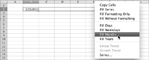
   Figure 1–23. To reach more AutoFill options, Ctrl+drag or right-drag the AutoFill handle, and then click the fill option you want on the context menu.

7. Click the Fill Months item, and Excel fills in a separate month for each column: 6/15/2011, 7/15/2011, and so on.

Now clear your data again and then create a sequence of numbers. Follow these steps:

1. Click cell A1 and type 5 in it.
2. Press Return to move to cell A2, type 25 in it, and press the up arrow to move back to cell A1.
3. Press Shift+down arrow to select cells A1 and A2.
4. Click the AutoFill handle and drag downward. AutoFill fills in a series with intervals of 20—cell A3 gets 45, cell A4 gets 65, and so on—using a linear trend.

Delete the data that AutoFill entered, leaving 5 in cell A1 and 25 in cell A2. Then follow these steps:

1. Select cells A1 and A2.
2. Ctrl+click or right-click the AutoFill handle and drag downward. As you drag, you'll see ScreenTips for the same values as in the previous list.
3. Release the mouse button and then click Growth Trend on the context menu. AutoFill enters a growth trend instead of the linear trend: because the second value (25) is 5 times the first value (5), Excel multiplies each value by 5, giving the sequence 5, 25, 125, 625, 3125, and so on.

Those are the basics of AutoFill. But you can also create custom AutoFill lists to quickly enter exactly the data you need.

Creating Your Own Custom AutoFill Lists

If you need to enter the same series of data frequently, follow these steps to create your own AutoFill lists:

1. If the data for the series already appears in a worksheet, select the cells that contain it.
2. Choose Excel Preferences or press Cmd+, (Cmd and the comma key) to display the Excel Preferences dialog box.
3. In the Formulas and Lists area, click the Custom Lists item to display the Custom Lists pane (shown in Figure 1–24 with settings chosen). If you selected cells in step 1, the references appear in the Import list from cells text box; move ahead to step 6.
   

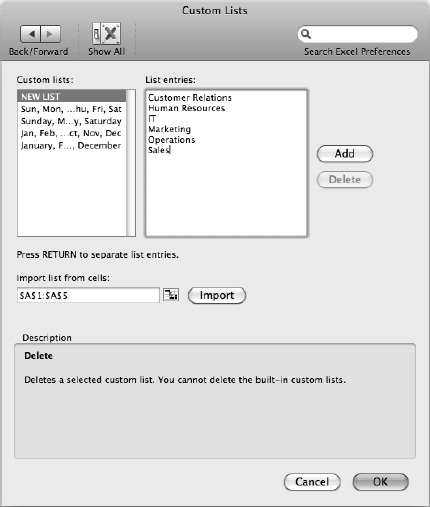
   Figure 1–24. You can supplement Excel's built-in AutoFill lists by creating your own data series.

4. In the Custom lists box, click the NEW LIST item.
5. Click in the List entries box, and then type your list, putting one item on each line.
6. If you've just entered a list, click the Add button to add the list to the Custom lists box. If you imported a list from a worksheet, click the Import button.

   TIP: If you need to create another list from worksheet data at this point, you don't need to close the Excel Preferences dialog box. Instead, click the Collapse Dialog button to the left of the Import button to collapse the Custom Lists dialog box to a shallow dialog box, then drag through the list on the worksheet. Click the Collapse Dialog button to restore the Excel Preferences dialog box, where the range appears in the Import list from cells text box. Then click the Import button to bring in the data.

7. Click the OK button to close the Excel Preferences dialog box.

Entering Text Using Paste and Paste Options

Often, you can enter text more quickly in your workbooks by pasting it in from other sources. For example, if you receive sales figures in an e-mail message, you can copy and paste them into a worksheet. To paste, select the upper-left cell of the range of cells into which you want to paste the data, and then give a Paste command—for example, click the Paste button on the Standard toolbar or press Cmd+V.

Excel lets you paste data in with or without all its formatting. Usually it's easiest to go ahead with a straightforward paste operation and then use the Paste Options action button (see Figure 1–25) to change the result if it's not what you want.

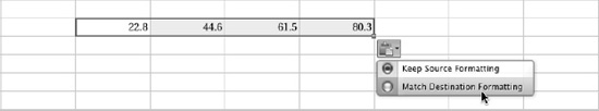
Figure 1–25. Use the Paste Options action button to switch pasted text from using its original formatting to matching the formatting of the destination.

When you paste in data you've copied from another application and you know you don't want to paste the formatting, use the Paste Special command like this:

1. Copy the data in the other application.
2. Switch to Excel.
3. Click the cell at the upper-left corner of the range you want to paste the data in.
4. Choose Edit Paste Special from the menu bar or Home Edit Paste Paste Special from the Ribbon (clicking the Paste pop-up button rather than the main part of the button) to display the Paste Special dialog box (see Figure 1–26).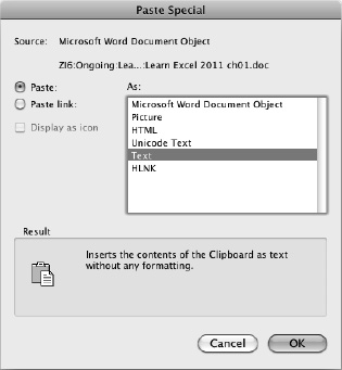
   

   Figure 1–26. Select the Text item in the As box in the Paste Special dialog box to paste in data from another application without pasting its formatting.

5. In the As box, click the Text item.

   TIP:If pasting using the Text item in the Paste Special dialog box puts all the text in one cell rather than in multiple cells, try using the Unicode Text item instead.

6. Click the OK button.

Switching Data from Rows to Columns

Often when you're laying out a worksheet, the best way to arrange the data isn't obvious at first—so you may find you've laid out your data out in rows when a column arrangement would work better.

Instead of spending hours retyping the data or using drag-and-drop to move it, you can fix the problem in moments using Excel's Transpose command. Follow these steps:

1. Make space for the transposed version of the data. Usually, it's easiest to put it on a separate worksheet; if so, click the Insert Sheet button to add one.
2. Select the data you want to switch from rows to columns.
3. Give a Copy command in any of the usual ways: Press Cmd+C, click the Copy button on the Standard toolbar, or choose Edit ä Copy from the menu bar.
4. Click the cell at the upper-left corner of the area into which you want to paste the transposed data.
5. Choose Home Edit Paste Transpose from the Ribbon, clicking the Paste pop-up button rather than the main part of the button. Excel pastes in the data, transposing its rows and columns.

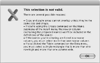
Figure 1–27. The This Selection Is Not Valid dialog box may indicate that you're trying to paste the transposed data back into its original location, an overlapping location, or a location that's the wrong shape.

Pasting in a Table from Word

If you have data in a table in Word, you can paste it straight into a worksheet in Excel. Excel places each table cell in a different worksheet cell, as you'd want.

You'll get the best results from a table that has a regular layout, with the same number of cells in each row. If some rows have more cells than other rows, you may need to move some cells in Excel after pasting them. In most cases, it's easiest to make the table regular in Word (for example, by making a copy of it in a spare document and the changing the copy) before pasting it into Excel.

Getting Comma-Separated Data into a Worksheet

If you have data in comma-separated format, you can get it into an Excel worksheet in three ways:

• Use the Text Import Wizard. As described earlier in this chapter, choose File Import, then use the Text Import Wizard to control exactly how Excel imports the text.
• Open the file in Excel. You can simply use the File Open command and the Open dialog box to open a comma-separated file in Excel. Excel automatically puts each comma-separated item in a separate cell. You can then copy and paste the data as needed.
• Convert the comma-separated data to a Word table, then paste it. If you have the data in comma-separated format as part of a document or e-mail message, follow these steps:
  1. Paste the data into a Word document.
  2. In Word, select the pasted data.
  3. Choose Table Convert Convert Text to Table from the menu bar to display the Convert Text to Table dialog box.
  4. In the Separate text at area, make sure the Commas option button is selected.
  5. Click the OK button. Word converts the text to a table.
  6. Select the table.
  7. Copy the table.
  8. Switch to Excel and paste in the table.

Pasting in Multiple Items with the Scrapbook

As you know, the Mac OS X Clipboard lets you store only one item at a time, so each time you copy something to the Clipboard, you overwrite its previous contents. But often you'll want to store various copied items so you can paste them whenever you need to. For example, you may want to store a graphics file containing your company logo or sections of boilerplate text that you need in many workbooks.

To let you store clippings and files in a single handy location from which you can paste them anywhere, Office:Mac provides the Scrapbook. The Office applications share the Scrapbook, so you can collect items in one application and use them in another.

Opening the Scrapbook

To open the Scrapbook, choose View Scrapbook from the menu bar or click the Toolbox button on the Standard toolbar and then click the Scrapbook button. Figure 1–28 shows the Scrapbook with several items stored in it. The left screen shows the Scrapbook's List view, the middle screen Detail view, and the right screen Large Preview.

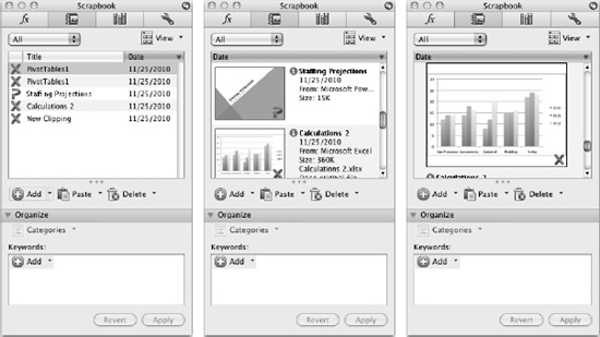
Figure 1–28. The Scrapbook can display its contents as a list (left), with details (middle), or as large previews (right). Use the View pop-up menu to switch views so that you can easily identify the item you want to paste.

Adding an Item to the Scrapbook

You can add an item to the Scrapbook in any of these ways:

• Add a selection. Select the text or other item you want to add to the Scrapbook. Then click the Add button in the middle of the Scrapbook palette.
• Add a graphics file. Click the Add drop-down button, then click Add File to display the Choose a File dialog box. Select the file you want and then click the Choose button.
• Add whatever you've copied to the Clipboard. Copy the item to the Clipboard as usual—for example, by selecting it in an application and then pressing Cmd+C. Then click the Add drop-down button in the Scrapbook palette and click Add from Clipboard.
• Add everything you copy to the Clipboard. If you use the Scrapbook extensively, you can make Office add a clipping of everything you copy in Mac OS X while the Scrapbook palette is open. To do so, click the Add drop-down button in the Scrapbook palette, then click Always Add Copy, placing a check mark next to this item. The application displays the Always Add Clipping Selected dialog box to warn you that this feature may slow your Mac down or take up disk space. Click the OK button.

Inserting an Item from the Scrapbook

To insert an item from the Scrapbook, select the cell or range in which you want to paste it. Then click the item in the Scrapbook palette and click the Paste button.

If you want to paste the item as plain text (without formatting) or as a picture, click the item and then click the Paste pop-up button. On the menu, click Paste as Plain Text or Paste as Picture, as needed.

Deleting an Item from the Scrapbook

Chances are you'll want to keep some items permanently in your Scrapbook, but you'll need to get rid of others when you no longer need them. Here's how to get rid of items:

• Delete a single item. Click the item, then click the Delete button.
• Delete all items currently displayed. Display the items you want to delete, click the Delete drop-down button, and then click Delete Visible.
• Delete all items from the Scrapbook. Click the Delete drop-down button, and then click Delete All.

Entering Text with Find and Replace

Excel includes a powerful Replace feature that you can use to replace text items in either the active worksheet or every worksheet in the active workbook. You can limit the search to matching the case you specify or by finding the match only as the entire contents of a cell rather than within a cell's contents.

To work with Replace, follow these steps:

1. Open the Replace dialog box (see Figure 1–29) in one of these ways:
   • Mouse. Click the pop-up button on the Search field on the Standard toolbar, then click Replace on the pop-up menu.
   • Menus. Choose Edit Replace.
   • Keyboard. Press Cmd+F to display the Find dialog box, then click the Replace button.
   

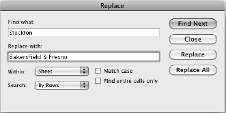
   Figure 1–29. You can use the Replace dialog box to quickly make changes throughout a worksheet or all the worksheets in a workbook.

2. Type the search term in the Find what box.
3. Type the replacement text in the Replace with box.
4. In the Within pop-up menu, choose Sheet if you want to replace instances of the search term only on the active worksheet. Choose Workbook if you want to replace items on all the sheets in the workbook.
5. In the Search pop-up menu, choose By Rows if you want to search across each row in turn. Choose By Columns if you want to search down each column in turn.
6. Select the Match case check box if you want to locate only instances that match the way you've typed the search term in the Find what box.
7. Select the Find entire cells only check box if you want to find only the cells whose entire contents match the search term. With this check box cleared, Excel also finds matches that form only part of a cell's contents.
8. Click the appropriate command button:
   • Find Next. Click this button to find the next instance of the search term so that you can decide whether to replace it.
   • Replace. Click this button to replace the instance that Excel has found and to find the next instance (if there is one). Lather, rinse, and repeat.
   • Replace All. Click this button to replace all the instances in the worksheet or workbook (depending on the setting you've chosen in the Within pop-up menu).
   • Close. Click this button when you've finished using the Replace dialog box.

Inserting Symbols in a Document

Just by typing, you can easily insert any characters that appear on your keyboard—but many documents need other symbols, such as letters with dieresis marks over them (for example, ë) or ligatures that bind two characters (for example, Æ).

You can quickly insert one or more symbols in a workbook by using the Symbol Browser pane in the Media Browser.

You can use the Symbol Browser pane in the Media Browser to insert a symbol in Word, Excel, or PowerPoint. To insert a symbol, follow these steps:

1. In the document, position the insertion point where you want the symbol to appear.
2. Choose Insert Symbol from the menu bar to display the Symbols pane of the Media Browser (see Figure 1–30).
   

   Figure 1–30 . To insert a symbol in a workbook, click the symbol in the Symbol Browser. Choose the All Symbols item in the pop-up menu to browse all symbols (left), or select only the set you're interested in (right).

3. Find the symbol you want in one of these ways:
   • Browse all symbols. Choose All Symbols in the pop-up menu at the top of the Symbol Browser, and then scroll down.

     TIP: Drag the slider at the bottom of the Symbol Browser to zoom in to enlarge the symbols, or zoom out to see more symbols at once.

   • Display only a set of symbols. Open the pop-up menu at the top of the Symbol Browser and click the set you want. For example, click the Greek set to display Greek characters.
4. Click the symbol to insert it in the document.
5. Leave the Symbol Browser open if you need to insert more symbols or other media objects. Otherwise, click the Media Browser's Close button (the button at the left end of the title bar) to close it.