Using Custom Views

When you need to keep your data laid out in a particular way, you can create a custom view. To do so, follow these steps:

1. Set up the workbook exactly the way you want it. For example:
   • Display the worksheet you want to see.
   • Hide any columns and rows you don't want to view. You'll learn how to hide columns and rows in Chapter 4.
   • Switch to the view you want.
   • Zoom the view as needed.
   • Set the print area.
   • Apply any filtering needed (see Chapter 10).
2. Choose View Custom Views from the menu bar to display the Custom Views dialog box (shown on the left in Figure 1–36 with two views already added).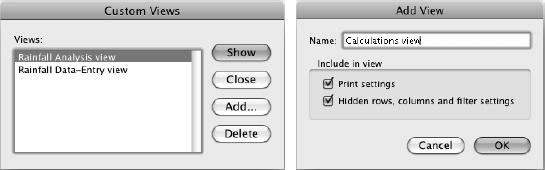
   

   Figure 1–36. Use the Custom Views dialog box (left) to add, delete, and display custom views. Use the Add View dialog box (right) to create a new custom view.

3. Click the Add button to display the Add View dialog box (shown on the right in Figure 1–36). Excel closes the Custom Views dialog box.
4. Type the name for the view in the Name text box.
5. Select the Print Settings check box if you want the view to include the current print settings.
6. Select the “Hidden rows, columns and filter settings” check box if you want the view to include hidden rows, hidden columns, and any filtering you've applied.
7. Click the OK button to close the Add View dialog box. Excel creates the view.

You can now switch to the view by choosing View Custom Views from the menu bar to display the Custom Views dialog box, clicking the view in the Views list, and then clicking the Show button.