Identifying Parts with Named Ranges

When you're setting up formulas in your workbooks, you'll often need to refer to particular cells and ranges. You can always refer to cells and ranges using their addresses, but these can be hard to remember—especially if you change their location by adding cells, rows, or columns to your worksheet.

To make your references easier to enter and recognize, you can give a name to any cell or range. You can then refer to the cell or range by that name. Excel tracks the current position of each name, so even if you add or delete cells (or rows or columns), you can still use the name without worrying about exactly where it is.

You can also use named ranges to navigate your worksheets easily: To go to a named range, open the pop-up menu in the reference area and click the range's name.

Assigning a Name to a Cell or Range

You can assign a name to a cell or range either quickly using the Reference Area or more formally using the Define Name dialog box. The advantage to using the Define Name dialog box is that you can manage your existing range names from there too.

These are the rules for creating names:

• The name must start with a letter or an underscore.
• The name can contain only letters, numbers, and underscores. It can't contain spaces or symbols.
• The name must be unique in the workbook.

Assigning a Name to a Cell or Range Quickly

To assign a name to a cell or range quickly using the Reference area, follow these steps:

• Select the cell or range you want to name.
• Click in the Reference area. Excel selects its current contents, which is the reference of the active cell (for example, B5).
• Type the name for the cell or range, and then press Return to apply it.

Assigning a Name to a Cell or Range with the Define Name Dialog Box

To assign a name to a cell or range using the Define Name dialog box, follow these steps:

1. Select the cell or range you want to name.
2. Choose Insert Name Define from the menu bar to display the Define Name dialog box (shown in Figure 3–13 with settings chosen).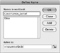
   

   Figure 3–13. In the Define Name dialog box, type the name you want to assign the cell or range so you can easily refer to it.

3. In the Name text box, type the name for the cell or range.
4. Make sure that the Refers to box shows the right cell or range. If not, click the Collapse Dialog button, select the right cell or range in the worksheet, and then click the Collapse Dialog button again to restore the dialog box.
5. If you want to create only this one name, click the OK button to apply the name to the range and close the Define Name dialog box. If you want to create more names before you close the Define Name dialog box, click the Add button.

Creating Range Names Automatically

If your worksheet has headings in the first column or last column or the first row or last row of an area, you can have Excel automatically create range names for you. This feature can save you time and effort.

When Excel creates the named ranges, it makes each an equal-sized section of the range you select. For example, if you create named ranges using the top row of the selection (A1:F5) shown in Figure 3–14, Excel creates a range named Stockton for cells B2:B5, a range called Modesto for cells C2:C5, and so on. Excel replaces spaces, punctuation, symbols and other characters in the headings that aren't allowed in names with underscores—for example, the heading City of Industry produces the name City_of_Industry.

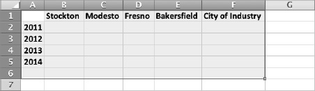
Figure 3–14. Creating named ranges using the headings in this selection produces ranges named Stockton for the range B2:B5, Modesto for the range C2:C5, and City_of_Industry for the range F2:F5.

To create names automatically, follow these steps:

1. Enter the headings in the worksheet.

   NOTE: In order to create names, each heading must begin with a letter rather than a number. So if you need to create names for cell containing (say) years, you need to preface the numbers with one or more letters—for example, Year 2011 rather than plain 2011.

2. Select the range that contains the headings. The headings must be in the top row, bottom row, left column, or right column of the selection.

   NOTE: When selecting the range from which to create labels, you must select more than one row (if the headings are in a row) or more than one column (if the headings are in a column). Otherwise, Excel displays the The Selection Is Not Valid dialog box. If this happens, click the OK button and change your selection.

3. Choose Insert Name Create to display the Create Names dialog box (see Figure 3–15).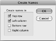
   

   Figure 3–15. In the Create Names dialog box, select the check box for each column and row that contains the headings you want to turn into range names.

4. In the Create names in box, select the Top row check box, the Left column check box, the Bottom row check box, and the Right column check box, as appropriate.
5. Click the OK button. Excel closes the Create Names dialog box and creates the names.

Excel doesn't display a dialog box or otherwise confirm that it has created the names. If you want to check that the names are there, open the pop-up menu on the Reference area and you'll see them in alphabetical order.

Using a Range Name in Your Formulas

After you name a range, you can use the name in your formulas instead of the cell reference or range reference. Named ranges can be a great time-saver, because names are much easier to remember and type than the cell references or range references.

For example, if you give a cell the name Interest_Rate, you can use it in a formula like this:

When your range names are straightforward like this, you may want to just type them in. Other times, you may find it easier to paste a name in like this:

1. Move the active cell to where you want the formula.
2. Start the formula as usual. For example, type =.
3. When you reach the part of the formula that needs the name, choose Insert Name Paste to display the Paste Name dialog box (see Figure 3–16).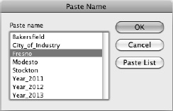
   

   Figure 3–16. Use the Paste Name dialog box to paste a range name into a formula. You can also paste the whole list of range names and their locations for reference.

4. In the Paste name list box, click the range name you want to paste.
5. Click the OK button. Excel closes the Paste Name dialog box and pastes in the name.

Deleting a Range Name

To delete a range name, follow these steps:

1. Choose Insert Name Define from the menu bar to display the Define Name dialog box.
2. Click the range name in the Names in workbook list box.
3. Click the Delete button.
4. Delete other range names as needed, then click the Close button to close the Define Name dialog box.

Changing the Cell or Range a Name Refers To

If you need to change the cell or range a name refers to, follow these steps:

1. Choose Insert Name Define from the menu bar to display the Define Name dialog box.
2. Click the existing name in the Names in workbook list box.
3. Triple-click in the Refers to box to select the current reference.
4. In the worksheet, click the cell or select the new range. (You can click the Collapse Dialog button first if you need to reduce the Define Name dialog box, but usually it's easier just to work around it.)
5. Click the OK button if you want to make the change and close the Define Name dialog box. Click the Add button if you want to make the change but keep the Define Name dialog box open.