
Working with Rows and Columns
In this section, you'll learn how to insert and delete rows, columns, and cells; change the width of columns and the height of rows; and hide rows or columns when you don't need to see them.
Inserting and Deleting Rows, Columns, and Cells
When laying out your worksheets, you'll often need to insert or delete entire columns or rows. Sometimes you may also need to delete a block of cells without deleting an entire column or row.
Inserting Columns and Rows
The easiest way to insert a column or row is to Ctrl+click or right-click the heading of the existing column or row before which you want to insert the new one and then click Insert on the context menu.
To insert more than one column or row, select the same number of columns or rows first. For example, to insert three columns before column F, drag through the headings of columns F, G, and H to select those columns; then Ctrl+click or right-click anywhere in the selected headings, and click Insert on the context menu.
You can also insert a column by selecting a cell in the column before which you want to add the new column, and then giving either of these commands:
- Ribbon. Choose
Home
Cells Insert Insert Columns. - Menu bar. Choose
Insert Columns.
NOTE: If the Excel window isn't wide enough for the Insert button, Delete button, and Format button to appear in the Cells group, an Actions pop-up button appears instead. Click this button to display a pop-up menu with an Insert submenu, a Delete submenu, and a Format submenu. Click the appropriate menu, and then make your choice from it.
Similarly, you can insert a row by selecting a cell in the row before which you want to add the new row and then giving either of these commands:
- Ribbon. Choose
Home Cells Insert Insert Rows. - Menu bar. Choose
Insert Rows.
As before, if you want to insert multiple columns or rows, select cells in the corresponding number of columns or rows first.
NOTE: What the Insert button in the Cells group on the Home tab of the Ribbon inserts depends on what you've selected. Select one or more columns to make the Insert button insert columns; select one or more rows to make the Insert button insert rows; or select one or more cells to make the Insert button insert cells. If you haven't selected the appropriate item, click the Insert pop-up button rather than the main Insert button, and then choose the item you want from the pop-up menu.
Inserting Some Cells
To insert just some cells, follow these steps:
- Select the range before which you want to insert the cells.
- Choose
Home Cells Insert Insert Cellsto display the Insert dialog box (see Figure 4–1).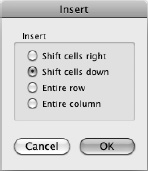
Figure 4–1. When you insert a block of cells, click the Shift cells right option button or the Shift cells down option button in the Insert dialog box to tell Excel which way to move the existing cells.
- Select the Shift cells right option button to move the existing cells to the right. Select the Shift cells down option button to move the existing cells down the worksheet. You can also select the Entire row option button to insert a whole row or select the Entire column option button to insert a whole column, but it's usually easier to insert a row or column by using the methods described earlier.
- Click the OK button to close the Insert dialog box. Excel inserts the cells.
Deleting Columns or Rows
The easiest way to delete a column or row is to Ctrl+click or right-click its heading, and then click Delete on the context menu. Alternatively, you can select the row or column and then choose Edit![]()
Delete from the menu bar or Home ![]()
Cells ![]()
Delete (clicking the main part of the Delete button) from the Ribbon.
Instead of selecting the column or row, you can click a cell in it, choose Home ![]()
Cells ![]()
Delete (clicking the Delete pop-up button), and then click Delete Columns or Delete Rows, as needed. Usually, it's easier to select the row or column first.
Deleting Some Cells
To delete just some cells, select them, and then choose Home ![]()
Cells ![]()
Delete ![]()
Delete Cells. In the Delete dialog box (see Figure 4–2) that Excel displays, select the Shift cells left option button or the Shift cells up option button, as appropriate, and then click the OK button.
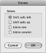
Figure 4–2. When you delete a block of cells, click the Shift cells left option button or the Shift cells up option button in the Delete dialog box to tell Excel how to fill the gap in the worksheet.
NOTE: In the Delete dialog box, you can select the Entire row option button to delete the row the selected cell is in, or select the Entire column option button to delete the column. This is useful when you realize you need to delete entire rows or columns rather than just a block of cells. Otherwise, you don't need to open the Delete dialog box to delete rows or columns.
Setting Row Height
Excel normally sets the row height automatically to accommodate the tallest character or object in the row. For example, if you type an entry in a cell, select the cell, and click the Increase Font Size button in the Font group of the Home tab a few times, Excel automatically increases the row height so that there's enough space for the tallest characters.
If Excel doesn't set the row height automatically, choose Home ![]()
Cells ![]()
Format ![]()
AutoFit Row Height to force automatic fitting.
Automatic row height works well for many worksheets, but you may sometimes need to set the row height manually. Use either of these ways:
- Drag the lower border of the row heading. Move the mouse pointer over the lower border of the row heading so that the pointer changes to an arrow pointing up and down, and then click and drag the border up (to make the row shallower) or down (to make the row deeper).
- Use the Row Height dialog box. Ctrl+click or right-click the row heading, and then click Row Height on the context menu to display the Row Height dialog box (see Figure 4–3). Type the row height you want, and then click the OK button.
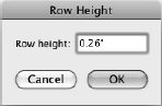
Figure 4–3. Use the Row Height dialog box when you need to set a row's height precisely.
NOTE: You can also display the Row Height dialog box by choosing Home ![]()
Cells ![]()
Format ![]()
Row Height from the Ribbon or Format ![]()
Row ![]()
Height from the menu bar.
Setting Column Width
Unlike with row height, Excel doesn't automatically adjust column width as you enter data in a worksheet. This is because many worksheets need long entries in cells, so automatic adjustment would make it hard to work.
You can quickly set column width in any of these ways:
- AutoFit a column. Double-click the right border of the column heading. Excel automatically changes the column's width so that it's wide enough to contain the widest entry in the column.
- AutoFit several columns. Select cells in all the columns you want to affect, and then double-click the right border of any of the selected column headings. Excel automatically fits each column's width to suit its contents. You can also select the cells and then choose
Home Cells Format AutoFormat Column Widthfrom the Ribbon orFormat Column AutoFit Selection.
TIP: AutoFit is usually the best way to resize a worksheet's columns. But if some cells have such long contents that AutoFit will create huge columns, set the column widths manually and hide parts of the longest contents. You can also wrap the text within a cell so that it occupies as many lines as it needs; you'll learn how to do this in the section “Setting Alignment” later in this chapter.
- Resize a column by hand. Drag the right border of the column heading as far as needed.
- Resize a column precisely. Ctrl+click or right-click the column heading, and then click Column Width on the context menu to display the Column Width dialog box (see Figure 4–4). Type the cell width, and then click the OK button.
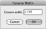
Figure 4–4. Use the Column Width dialog box when you need to set the column width precisely.
- Resize several columns precisely to the same width. Select the columns by dragging through their column headings or by selecting cells in each column. Ctrl+click or right-click in the selected column headings, then click Column Width on the context menu to display the Column Width dialog box. Type the column width and then click the OK button.
Hiding Rows and Columns
Sometimes it's helpful to hide particular columns and rows so that they're not visible in the worksheet. You may want to do this to keep sensitive data from showing or simply to make the part of the worksheet you're actually using fit on the screen all at once.
To hide a column or row, Ctrl+click or right-click its column heading or row heading and then click Hide on the context menu. You can also click a cell in the row or column and choose Home ![]()
Cells ![]()
Format ![]()
Hide Row or Home ![]()
Cells ![]()
Format ![]()
Hide Column from the Ribbon or Format ![]()
Row ![]()
Hide or Format ![]()
Column ![]()
Hide from the menu bar.
TIP: To quickly hide the active row or selected rows, press Ctrl+9. To hide the active column or selected columns, press Ctrl+0.
To unhide a row or column, select the rows above and below it or the columns on either side of it. Then Ctrl+click or right-click the selected row headings or column headings and click Unhide on the context menu.
NOTE: You can also hide and unhide items by choosing Home ![]()
Cells ![]()
Format ![]()
Unhide Row or Home ![]()
Cells ![]()
Format ![]()
Unhide Column from the Ribbon or by choosing Format ![]()
Row ![]()
Unhide or Format ![]()
Column ![]()
Unhide from the menu bar.