Using Data Bars

A data bar is a horizontal bar that appears in a cell to graphically represent the value in a corresponding cell. Normally, you'll use data bars to represent the values of multiple cells so that you can see the relationship among the cells' values.

For example, the worksheet in Figure 8–1 uses data bars to show the sales by five different salespeople for April, May, June, and the second quarter of the year as a whole. Each cell that contains a data bar has the same value as the cell to its left, so the data bar in cell C2 illustrates the value shown in cell B2. Looking at the data bars, you can easily see that although Salesperson Smith had a weak April and a shoddy May, her strong June sales brought her up to a respectable result for the quarter overall.

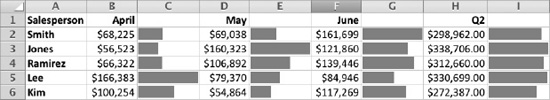
Figure 8–1. Data bars give a quick graphical representation of the values in the cells. Here, each cell showing a data bar contains the same value as the cell to its left.

Creating Data Bars

By default, Excel places data bars alongside the data they represent. You can choose to display only the data bars in the cells, or you can display the data bars in separate cells to make the worksheet easier to read.

Creating Data Bars in the Same Cells as Their Data

To create data bars that appear in the same cells as their data, follow these steps:

1. Enter the data from which you'll create the data bars. If the data is already in the worksheet, you're all set.
2. Select the cells that contain the data.
3. Choose Home Format Conditional Formatting Data Bars to display the Data Bars panel (see Figure 8–2).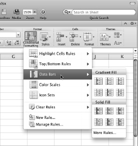
   

   Figure 8–2. Use the Home Format Conditional Formatting Data Bars command to create data bars in the selected cells. You can choose between a gradient fill and a solid fill.

4. Click the color and fill type you want in either the Gradient Fill section or the Solid Fill section of the Data Bars panel. Excel creates the data bars in the cell. The left screen in Figure 8–3 shows an example.

   TIP: A gradient fill works best for data bars you display in the same cells as their data, because the lighter end of the gradient leaves the text readable. For data bars you display in cells on their own, you may prefer solid fills.

   

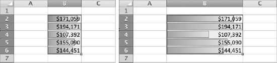
   Figure 8–3. After creating data bars (left), you may need to widen the column to give them more impact (right).

5. Change the column width if necessary. For example, drag the right border of the cell's column heading to the right to make the column wider and give the data bars more impact, as shown on the right in Figure 8–3.

Creating Data Bars in Different Cells Than Their Data

To make your data bars easy to read, you may want to have them appear in cells on their own, either with the underlying data appearing in cells alongside them (or elsewhere, as needed) or without the data appearing at all. You can make the data bars appear on their own in cells by setting Excel to display only the data bars there. If you want the data for the data bars to be visible, you need to place it in different cells.

To make the data bars appear without their data, follow these steps:

1. Create the data bars as described in the previous section, so that the data bars appear in the same cells as their data.
2. With the cells still selected, choose Home Format Conditional Formatting Manage Rules to display the Manage Rules dialog box (see Figure 8–4).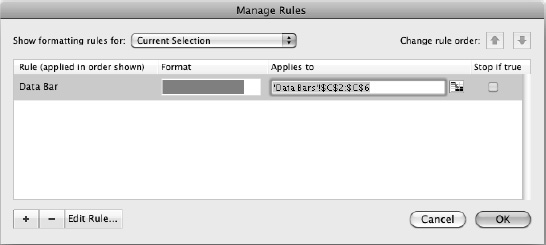
   

   Figure 8–4. In the Manage Rules dialog box, select the rule for the data bars, then click the Edit Rule button.

3. Make sure the right rule is selected. If you've applied only one conditional formatting rule to the cells, it will be selected; if you've applied multiple rules, you may need to select the right rule.
4. Click the Edit Rule button to display the Edit Formatting Rule dialog box (see Figure 8–5).
   

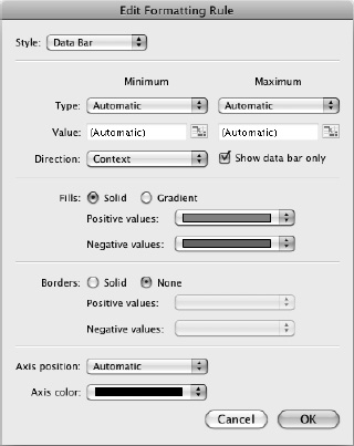
   Figure 8–5. In the Edit Formatting Rule dialog box, select the Show data bar only check box if you want to display the data bars without the values that produced them.

5. Select the Show data bar only check box.
6. Click the OK button to close the Edit Formatting Rule dialog box.
7. Click the OK button to close the Manage Rules dialog box.

To create data bars that appear in separate cells from the values that produce them, set up the cells that will contain the data bars with formulas referring to the cells that contain the values. For example, the worksheet shown in Figure 8–6 uses simple formulas such as =B2 to make the cells in column C have the same values as the cells in column B. You can then set up the data bars as described earlier in this chapter in the target cells—in this case, in column C.

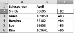
Figure 8–6. When you need to produce data bars in cells separate from their data, use formulas to give the data-bar cells the same values as the cells that provide the data. For example, cell C2 here contains the formula =B2 and will show the data bar for the value in cell B2.