
Showing Data Trends with Sparklines
As you saw in Chapter 7, charts are great for illustrating medium to large quantities of information, but sometimes you'll want something smaller—a chart that'll fit inside a single cell, giving a quick visual indication of a trend. Excel calls such charts sparklines.
Excel provides three kinds of sparklines:
- Line. A line sparkline is a straightforward line that runs through the data points, as in the top part of Figure 8–13. A line sparkline is good for showing data that flows from one data point to the next, such as temperatures.
- Column. A column sparkline shows the data as a series of columns, as in a column chart. The middle part of Figure 8–13 shows an example. A column sparkline is good for comparing data points that are separate from each other, such as sales results by month.
- Win/Loss. A win/loss sparkline shows results as either a win (a positive result) or a loss (a negative result). The lower part of Figure 8–13 shows an example of win/loss sparklines. A win/loss sparkline is good for when you want to take a black-and-white view of results—for example, whether your investments are up or down in a particular month. In a win/loss sparkline, a zero value appears as a blank.
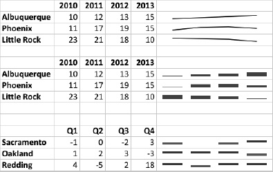
Figure 8–13. Sparklines are single-cell charts that you can use to indicate trends or results visually.
Inserting Sparklines
To insert one or more sparklines in a worksheet, follow these steps:
- Click the cell or select the range you want to place the sparklines in.
- Click the Charts tab to display its contents, go to the Insert Sparklines group, then click the Line button, the Column button, or the Win/Loss button, as needed. Whichever button you click, Excel displays the Insert Sparklines dialog box (see Figure 8–14).
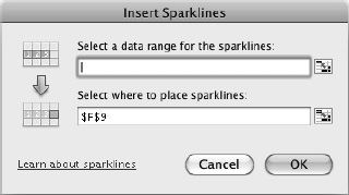
Figure 8–14. In the Insert Sparklines dialog box, choose the data range for the sparklines and the cells in which to place them.
- With the focus in the Select a data range for the sparklines text box (where Excel places it when it displays the Insert Sparklines dialog box), click and drag in the worksheet to enter the range that contains the data for the sparklines.
- Make sure the Select where to place sparklines text box contains the range in which you want to place the sparklines. If you chose the range before displaying the Insert Sparklines dialog box, it'll be correct. Otherwise, click in this text box, then drag in the worksheet to select the range.
- Click the OK button to close the Insert Sparklines dialog box. Excel inserts the sparklines in the cells.
Formatting Your Sparklines
After inserting sparklines, you can format them by using the controls on the Sparklines tab of the Ribbon. Click a cell in the sparklines to select the group of sparklines and make Excel add the Sparklines tab to the Ribbon. If Excel doesn't display the Sparklines tab automatically, click the tab to display it (see Figure 8–15).

Figure 8–15. Use the controls on the Sparklines tab of the Ribbon to format sparklines to look the way you want them to.
These are the main moves for formatting your sparklines:
- Change the source data for a group of sparklines. Click a cell in the group of sparklines, then choose
Sparklines
Data Editfrom the Ribbon (clicking the main part of the Edit button). Excel displays the Edit Sparklines dialog box, which has the same controls as the Insert Sparklines dialog box. - Change the source data for a single sparkline. Click the sparkline cell, then choose
Sparklines Data Edit Edit Single Sparkline. Excel displays the Edit Sparkline dialog box, which works like the Insert Sparklines dialog box, but affects only the cell you chose. - Change a sparkline to a different type. Click the sparkline cell, then click the Line button, the Column button, or the Win/Loss button in the Change Type group on the Sparklines tab of the Ribbon.
- Add markers to the sparklines. In the Markers group on the Sparklines tab of the Ribbon, select the High check box, the Low check box, the Negative check box, the First check box, or the Last check box as needed—or select the All check box to select all the others. To change the marker color, choose
Sparklines Format Markers, then work in the Markers dialog box (see Figure 8–16).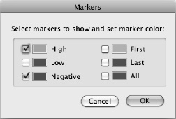
Figure 8–16. Use the Markers dialog box to change the colors of markers and to choose which ones appear on the sparklines.
- Apply a style to the sparklines. In the Format group on the Sparklines tab of the Ribbon, either click a style in the Styles box or hold the mouse pointer over the Styles box to display the panel button. Next, click the panel button to display the Styles panel, then click the style you want.
- Change the color of the sparklines. Choose
Sparklines Format Sparklineto display the Sparkline panel, then click the color you want. - Change the weight of the sparklines. Choose
Sparklines Format Sparkline Weight, then click the line weight. - Change the axes for the sparklines. Choose
Sparklines Format Axesto display the Axes dialog box (see Figure 8–17), then make your choices in it.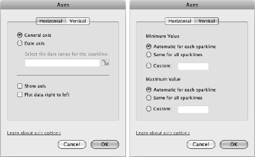
Figure 8–17. You can use the Axes dialog box to choose settings for the horizontal and vertical axes of the sparklines.
- Group sparklines together. If you need to format separate sets of sparklines quickly, group them together. Select each set of sparklines, then choose
Sparklines Edit Groupfrom the Ribbon to group them. - Clear sparklines. When you no longer need sparklines, clear them from the cells. Select the sparkline cells you want to clear, then choose
Sparklines Edit Clear, clicking the main part of the Clear button. You can also click a single cell and then chooseSparklines Edit Clear Clear Selected Sparkline Groupsto clear all the cells in the group