
Flipping Across the Axis
Whether you are working with a linear or a non-linear equation, a negative coefficient has the effect of reversing the slope of the graph. A typical scenario with a linear equation involves seeing the line change so that instead of going from quadrant III to quadrant I, the line goes from quadrant II to quadrant IV. With a parabola, you see the vertex of the parabola flipped so that it opens downward.
Linear Flips
To use Visual Formula to show how changing the coefficient of a variable alters the slope or orientation of a graph, you can start out by working with a linear equation and generating a graph of a line with a positive slope. Then you can create a line with a negative slope. The following sections review the necessary steps. Refer to Figure 10.32 as you go.
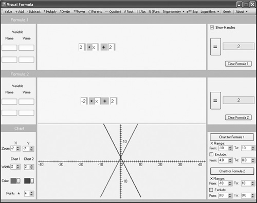
Figure 10.32. A line with a positive slope crosses a line with a negative slope.
The Positive Slope
Assume you are working with an equation that takes the form y = m (x)+ b. To implement this equation, work in the top equation composition area. Use the following steps:
Click the menu item for Value. Then click in the equation composition area to position the Value field. Type 2 in the Value field. This is the field that corresponds to the coefficient m.
Click the Multiply menu item. Then click to the right of the Coefficient field to position the multiplication sign.
Click the Value field again and position the field to the right of the multiplication sign in the equation composition area. Type x in this field.
Click the Add menu item and position the plus sign to the right of the x field.
Click to activate the Value menu item. Click after the plus sign to position the field. This is the field for the y-intercept value. Type 2 in the field.
Now go to the lower-right panel and find the To and From fields for the X Range setting. Click the To control and set the value of the field to –10. Click the From control and set the value of the field to 10.
On the Chart panel, find the Zoom fields. Click the x axis control and set the value of –7. Likewise, click the y axis control and set the value to –7.
Also, for the Width values, use the controls to set the Chart 1 and Chart 2 values to 2.
Now click the Chart for Formula 1 button. As Figure 10.32 illustrates, a graph of a linear equation with a positive slope of 2 and a y-intercept of 2 appears in the Cartesian plane.
The Negative Slope
In the previous section, you generated a line with a positive slope. Now complement this work by generating a line with a negative slope. The equation you work with in this instance assumes the form y = –m (x)+ b. To implement this equation, work in the lower equation composition area. Use the following steps:
Click the menu item for Value. Then click in the lower equation composition area to position the Value field. Type –2 in the Value field. This is the field that corresponds to the coefficient m. The minus sign establishes a slope opposite of the one you implemented previously.
Click the Multiply menu item. Then click to the right of the Coefficient field to position the multiplication sign.
Click the Value field again, and position the field to the right of the multiplication sign in the lower equation composition area. Type x in this field.
Click the Add menu item, and position the plus sign to the right of the x field.
Click the Value menu item, and then position the Value field after the plus sign. This is the field for the y-intercept value. As before, type 2 in the field.
Now go to the lower-right panel and find the To and From fields for the X Range setting beneath the Chart for Formula 2 button. These values should already be set to correspond with those of the Chart for Formula 1 button, but to verify that this is so, click the To control and set the value of the field to –10. Click the From control and set the value of the field to 10.
Now click the Chart for Formula 2 button on the right. You can also click the Chart for Formula 1 button to refresh the previous graph. Graphs of the equations with slopes –2 and 2 and y-intercept 2 appear in the Cartesian plane. As Figure 10.32 illustrates, the negative slope slants down to the right.
Absolute Value Flips
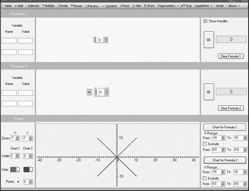
An equation for an absolute value takes the form y = |x|. Such an equation generates a graph in a V shape. The vertex of the V opens upward. To flip this graph so that its vertex opens downward, you introduce a negative slope. The form of the equation becomes y = –m|x|. Figure 10.33 illustrates two graphs of equations that possess absolute values. The V above the x axis represents a positive slope. The V below the x axis represents a negative slope.
Figure 10.33. You can flip the graphs of equations containing absolute values if you multiply by a negative value.
To use Visual Formula to implement these two equations, use the following approach:
Click the Abs (absolute value) menu item. Then click in the upper equation composition area to position the absolute value bars. Pull the bars apart so that they can accommodate a variable.
To generate the graph of this absolute value equation, locate the Chart for Formula 1 button in the lower-right panel and click on it. You see the graph that appears above the x axis in Figure 10.33.
To implement an absolute value function that generates the inverted graph shown in Figure 10.33, follow these steps:
Click the Subtract menu item. To position the minus sign the Subtract menu generates, click in the lower equation composition area.
Click the Abs (absolute value) menu item. Then click in the lower equation composition area to the right of the minus sign to position the absolute value bars. Pull the bars apart far enough to accommodate a variable.
Click the Value menu item. To position the Value field, click between the absolute value bars.
Now click the Chart for Formula 2 buttons to see the graph. This graph appears below the x axis.
To give your graphs the appearance of those illustrated in Figure 10.33, use the following approach:
Locate the X Range fields below both of the Chart for Formula 1 and Chart for Formula 2 buttons. These are in the lower-right panel.
Click the arrow controls for the From fields and set them to –10.
Click the arrow controls for the To fields and set them to 10.
On the Chart panel, set the x and y Zoom values to –7. Set the Width fields for both charts to 2.
Finally, set the Points field to 2.
Flipping Parabolas
To flip a parabola, you provide a negative value as the coefficient of x. Consider, for example, the equation y = x2. You can rewrite this equation as y = ax2. In this instance, the constant a equals 1, so if you make the equation explicit, then it reads y = (1)x2. The value of the coefficient is 1, and the coefficient defines how the vertex of the parabola the equation generates opens. A positive value makes it open upward.
If you change the equation so that the value of the coefficient becomes negative, then the equation takes on this form: y = (–1)x2. When you make the coefficient negative, you change the way the parabola opens. It now opens downward.
To put Visual Formula to work to implement an equation that generates a parabola that opens upward, you implement the equation that reads y = (1)x2. To accomplish this task, use the following steps:
Click the menu item for Value. To position the Value field, click in the upper equation composition area. Type x in the Value field.
Then, to create an exponent, click the Power menu item. To position this field, click to the upper right of the Value field. After you position the Exponent field, type 2 in it.
To generate the graph of the equation, proceed to the lower-right panel and click the Chart for Formula 1 button. As illustrated in Figure 10.34, you see a parabola that opens upward from the x axis.
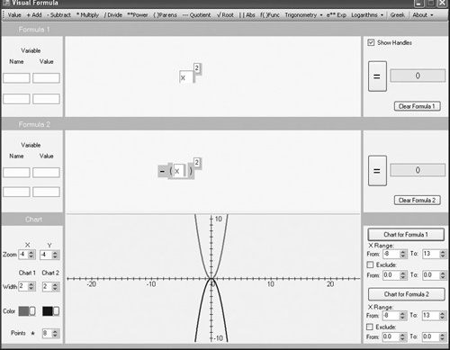
Figure 10.34 illustrates a second parabola, one that opens downward. You can express the equation that generates this parabola as y = (–1)a2. Use these steps in Visual Formula to implement the equation:
Click the menu item for Subtract. Then click in the lower equation composition area to position the minus sign that corresponds to the Subtract menu item.
Next, click the Parens menu item. Click after the minus sign to position the parentheses, and then pull them far enough apart to accommodate a Value field.
Click the Value menu item. Click inside the parentheses to place the corresponding field. Type x in the Value field.
Click the Power menu item. To position the Exponent field, click to the upper right of the closing parenthesis. After you position the Exponent field, type 2 in it.
To generate the graph, in the lower-right panel of Visual Formula, click the Chart for Formula 2 button.