
Linear Graphs
A linear function generates a graph characterized by a slope that does not change. The line-slope-intercept equation provides a way to experiment with linear equations. Here is the line-slope-intercept equation as you have seen it in previous chapters:
f (x) = mx + b or y = mx + b
Drawing from Table 10.1, you can use this equation to generate a line with a positive slope of 2 and a y-intercept at 3:
y = 2x + 3
| Item | Discussion |
|---|---|
| y = 2x + 3 | Creates an equation that slopes upward into quadrant I with the y-intercept at 3. |
| Creates a line that is perpendicular to the line you create with y = 2x + 3. |
| Reduces the severity of the slope you generate with y = 2x + 3. |
| y = –2x + 3 | Causes the slope to trail downward from quadrant II to quadrant IV. Passes through quadrant I from the y-intercept at 3. |
| y = 2x – 3 | Moves the y-intercept below the x axis. The line you generate in this way parallels the line you generate with y = 2x + 0. |
| y = –2x – 3 | Reverses the slope and places the y-intercept below the x axis. |
| y = 2x + 0 | Causes the line to cross the origin of the Cartesian system (value of the y-intercept is 0). The line remains perpendicular to |
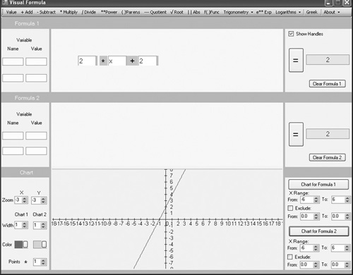
Refer to Figure 10.1 as you go, and implement this equation in Visual Formula using the following steps:
Click the Value menu item. To position the field the Value menu activates, click in the top equation composition area. This creates a field for constants that corresponds to the m constant. This constant defines the slope of the equation. For the value for the field, click in the box and type 2.
Click the Multiply menu item. Then click to place the multiplication symbol immediately after the Value field.
After setting up the Value field for x, click the Add menu item. To place the plus sign in the equation composition area, click just after the x Value field.
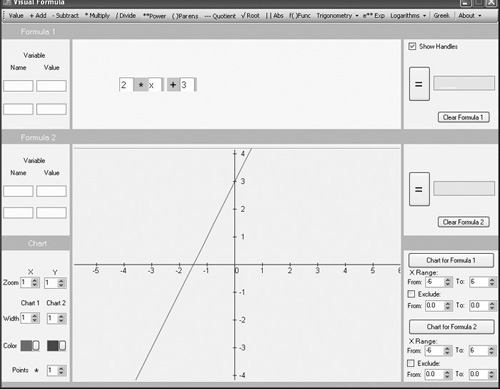
See the equation composition area of Figure 10.1 for the appearance of the equation after you have implemented it. To test your work, click the button on the right of the composition that contains the equal sign. You see 2 in the field adjacent to it.
Now you can proceed to generate a graphical representation of the equation. Toward this end, first move the cursor to the top of the Cartesian plane. As you do so, the cursor turns into a horizontal line with arrows extending up and down. Press the left mouse button and pull the Cartesian plane upward until its top edge is even with the bottom of the composition area that contains your equation. Figure 10.1 illustrates Visual Formula after you have extended the Cartesian plane.
Having extended the Cartesian plane, you are ready to generate the line. To accomplish this, click on the Chart for Formula 1 button on the lower right panel of the Visual Formula window. You see the line illustrated in Figure 10.1.
Changing the Intercept Value
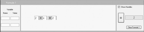
To work with the linear equation you have set up in the previous exercise, find the y-intercept field in your equation in the composition area. You have assigned an initial value of 3 to the y-intercept. The value corresponds to the b constant in the slope-line-intercept equation. The goal here involves altering this value to see the difference that results in the position of the line.
Referring to Figure 10.2, change the value of the y-intercept to 3. To do so, click to activate the field. Press the back arrow key to delete the previous value. Type 2 to replace it. To verify your value, click the button with the equal sign on the right. The value you see is 2, as Figure 10.2 illustrates.
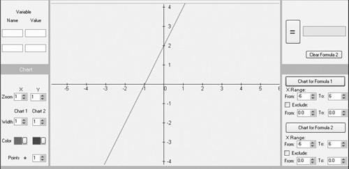
Now click the Chart for Formula 1 button in the lower-right panel. The position at which the line crosses the y axis changes. You see the line intercept with 2 on the y axis, as Figure 10.3 illustrates. After changing the y-intercept to 2, change it back to 3. Try other values, such as 1 and 4.
Figure 10.3. When you change your y-intercept value, you change the point at which the line intersects with the y axis.
Changing the Scale
Prior to proceeding with further operations, find the Zoom fields in the Chart panel (see Figure 10.4). The Zoom fields allow you to adjust the number of crosshatches you see on the x and y axes. In this instance, adjust the settings of both of the fields so that you see values of –3. Figure 10.5 illustrates the fields after you have adjusted the values. If you compare Figure 10.3 with Figure 10.5, you can see the scale of the lines is now much finer than before. The number of cross hatches on both axes increases.
Figure 10.4. Adjust the Zoom fields so that you see more points on the x and y axes.
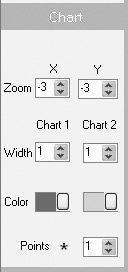
Figure 10.5. Adjust the Zoom fields so that you see more points on the x and y axes.
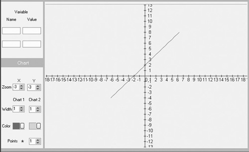
To explore the use of the Zoom controls, adjust the scale up and down. As long as you adjust the two controls in tandem, the appearance of the slope does not change. Figure 10.5 illustrates the Zoom controls set with values of –3. Positive values draw the crosshatches farther apart. Negative values draw them closer together.
Setting Up a Contrasting Line
To make it so that you can contrast the work of one equation with that of another, you make use of the upper and the lower equation composition areas. If you have performed the exercises in the previous sections, you have pulled the Cartesian plane over the lower composition area. You did this in part to be able to adjust the scale of the crosshatches on the axes. Now that you have adjusted the lines to accommodate your work, you can pull the Cartesian plane back so that it no longer conceals the lower equation composition area.
Toward this end, position the cursor on the top of the Cartesian plane until it appears as a horizontal bar with arrows extending up and down. Then press the left mouse button and pull downward on the bottom edge of the lower composition area. Pull it until it is even with the Chart panel, as shown in Figure 10.6.
Figure 10.6. Pull the lower equation composition area open above the Cartesian plane.
Now you have two equation composition areas to work with. The equation you created before is still in the upper equation composition area. The lower composition area remains blank.
To create a contrasting equation, consider another of the equations in Table 10.1:
![]()
Since the slope of this equation is ![]() , the line it generates appears more horizontal than a line with the slope of 2. To see how this is so, implement this equation in the lower equation composition area. Refer to Figure 10.7 and use the following steps:
, the line it generates appears more horizontal than a line with the slope of 2. To see how this is so, implement this equation in the lower equation composition area. Refer to Figure 10.7 and use the following steps:
Click the Value menu item. Then in the lower equation composition area, click to position the Value field. As in the previous exercise, this field corresponds to the m constant. This constant defines the slope of the equation. Type
 in this field. When you type this value, type 1, a forward slash (/), and then 2.
Click the Multiply menu item. Then click to place the multiplication symbol immediately after the Slope field.
Following the multiplication symbol, click the Value menu item. To place the second Value field, click to the right of the multiplication sign. Type an x in this field. The x represents a range of values Visual Formula can use to generate the graph of a line.
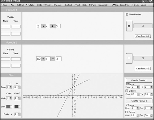
Having implemented the equation, click the Chart for Formula 2 button. As Figure 10.7 illustrates, the shorter, more gradually sloped line appears. To change the color of the line, click Color option on the Chart panel and select from the color palette.
You can use a similar approach to generate graphs for other linear equations. Table 10.1 provides some of the common forms of linear equations. Work through the examples the table provides.
Note
If you want to delete an element you have placed in the equation composition area, hold down the Shift key and click on the element.