Quadratic Equations

A quadratic equation is a polynomial of the second degree. In other words, one of its terms possesses an exponent of 2. A quadratic equation usually consists of three terms. Here is the standard form of a quadratic equation:

ax² + bx + c = 0

In such an equation, the constant a cannot be equal to 0, because then the variable x is also 0. As already mentioned, the degree of the quadratic equation is based on the value of the exponent for the variable x, which is 2. On the other hand, the constants c and b can be zero.

To solve quadratic equations, you can employ a set of techniques. Using this set of techniques provides a much easier way to solve quadratic equations than if you approach them intuitively. To understand how to use these techniques, consider working with the following equation:

x² = 36

Such an equation falls into the standard quadratic category, but to see it as such, you must realize that b and c are equal to zero. Think of the equation as

x² + 0x – 36 = 0

Since little is accomplished by using the second term, you can drop it. You are then left with this equation:

x² – 36 = 0

To solve for the value of x, you can draw from the discussion in Chapter 8 and factor the equation. To factor the equation, you draw on observations concerning the difference of two squares. You take the square roots of both of the terms in the expression. Accordingly, while x · x = x², it also stands that . If you then rearrange the resulting term so that you show the difference of two squares, your work appears as follows:

To generalize then, solving for the two terms, and , it is necessary to consider a set of observations that apply to the solutions of all quadratic equations. These observations are as follows:

• If the value of a is greater than zero, then there are two solutions .

• If the value of a equals zero, then only one solution is correct.

• If the value of a is less than zero, no solution exists. (You cannot in this situation find the square root of a negative number.)

Quadratic Appearances

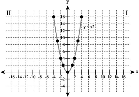
You can draw on the discussion that previous chapters provided to explore a few basic ideas that apply to representing quadratic equations. Consider, for example, that quadratic equations possess a degree of 2. A variable with an exponent of 2 represents a square. When you graph values you generate using a square, the values you generate are positive. For this reason, in the functional form of a quadratic equation, the values of a domain (x) generate positive values of a range (y). The resulting geometrical representation for this graph is a parabola. Figure 9.1 illustrates a parabola generated by the equation y = x².

The graph you generate using a quadratic equation differs from the graph you generate using a linear equation. The most fundamental characteristic of this difference is that the slope of a parabola changes, whereas that of a straight line defined by a linear equation does not.

To review this notion, consider the slopes shown in Figure 9.2. The slope of the parabola tends to become steeper the larger the value of y becomes. On the other hand, the slope of the linear equation remains constant throughout. The capacity to show the change in the slope of a line provides you with a powerful tool with which to examine rates of change. Central to this idea is that, as the value of the x axis increases, you can discern a continuously steeper or more accentuated change in the value of the yaxis. With change comes a change in the rate of change.

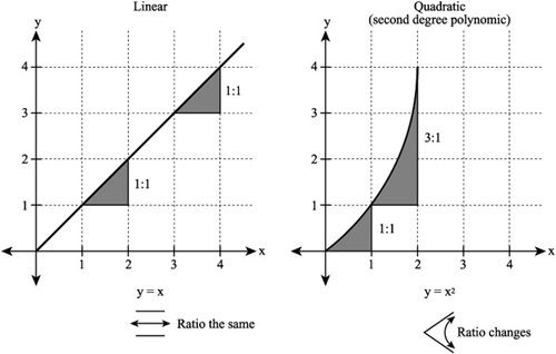
As Figure 9.2 reveals, the change of the slope reveals a changing relationship between the base number and the resulting value of y. Contrast what happens if you add 2 to 2 or 3. Each time, you perform the same action. You add 2 to a number. The slope of the graph that represents this activity stays the same. This activity differs from what happens when you employ an exponent.

When you employ an exponent, if you raise 2 to the power of 2, the relation between 2 and the base number changes as you increase the value of the exponent. With each successive exponential operation, the ratios between the values of x and y change, and the shape of the curve changes. When you can change the slope in this way, you arrive at a way of representing or describing phenomena that significantly expands the work you perform using linear equations.

Changing Appearances

The work you performed in Chapter 7 when examining absolute values anticipates the work you perform with quadratic equations. As Figure 9.3 illustrates, you can view the V shape of the graph you generate when working with absolute values as similar to the rounded U shape you generate when you work with quadratic equations. In both cases, the graph is symmetrical with respect to an axis. Two lines meet to form the vertex of an angle. In the same way the point that corresponds to the lowest (or highest) reach of the parabola is called the vertex of the parabola.

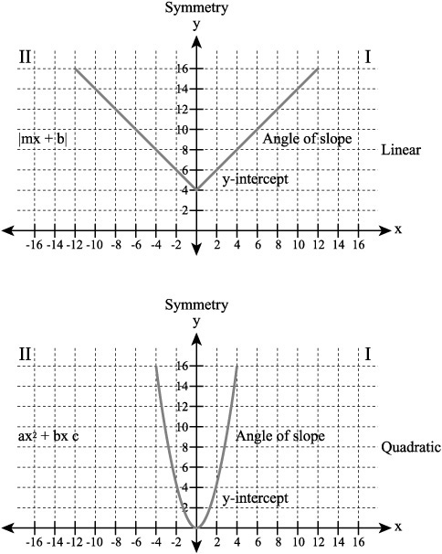
In most cases, the figures you generate are symmetrical with respect to the y axis, but you can also generate graphs that are symmetrical with respect to the x axis. Generally, however, if you apply the vertical line rule to the graph of a quadratic equation, then functions you define using quadratic equations remain symmetrical with respect to the y axis.

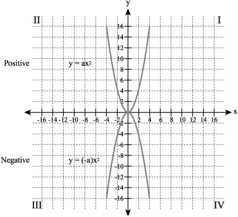
Positive and Negative

As with a linear equation generated using absolute values, a quadratic equation possesses attributes that allow you to adjust the appearance of the graph in a number of ways. In the most basic form of a quadratic equation, the vertex of the parabola opens upward and the parabola is symmetrical to the y axis. You can alter this situation if you apply a negative coefficient to the x variable of the quadratic. Figure 9.4 illustrates the effect of a negative coefficient. On the top, the parabola opens upward. The coefficient of x establishes a positive slope, so the parabola opens upward. On the bottom, the coefficient is negative, and the result is that the values you generate establish a negative slope. The parabola opens downward.

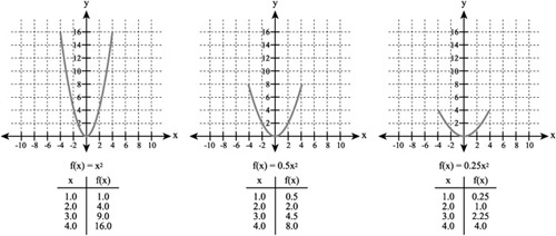
Widening a Parabola

As you can change a quadratic equation so that its vertex opens up or down, so you can change the width of a parabola. As with direction of the vertex, you adjust the coefficient of the x in a quadratic to change the width. If you make the value of the equation less than 1, then the parabola becomes less steep. Its mouth widens. Its rate of climb becomes less pronounced. Figure 9.5 illustrates this situation. On the left, you see a parabola defined with a coefficient of 1. In the middle, the value of the coefficient becomes . On the right, the value of the coefficient becomes As the value of the coefficient decreases, the slope of the line tends to become more gradual.

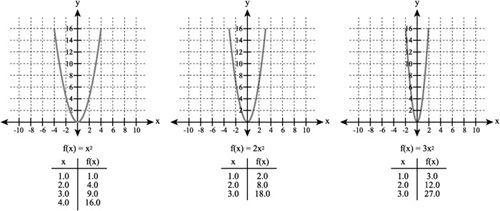
Narrowing a Parabola

As you might expect after experimenting with values less than 1 in relation to the coefficient of x in a quadratic equation, when you make the coefficient of x greater than 1, you increase the steepness of the parabola’s climb (or slope). Figure 9.6 illustrates how this happens. On the left, the parabola you see is defined by an equation in which the coefficient of x is 1. In the center, the value of the coefficient increases to 2. The steepness of the climb increases. On the right, the value of the coefficient increases to 3. The steepness of the climb becomes even greater. In each case, as the value of the coefficient increases, the steepness of the parabola becomes more pronounced.