Linear Functions

Certain functions are linear. A linear function is a function that generates a straight line. Here are a couple of examples of linear equations:

y = 2x + 3

4a – 3a = 12

Generally, when you formally identify such equations, you use the following expressions:

y = mx + b

Ax + By = C

In these equations, y and x represent variables. You can view x as representing the domain value and y as representing the range value. In both cases, these are variable values. The other letters (m, b, A, B, and C), represent constant values. A constant value is a value you see literally expressed. In the first equation, 2 and 3 serve as constants. In the second equation, 4 and 3 furnish the constants.

The equation y = mx + b is known as the slope-intercept equation. The variable m identifies the slope. The letter b identifies the y-intercept. Here’s yet another rewriting of the equation:

value_of_range = slope (value_of_domain) + y-intercept

Table 6.1 provides discussion of the primary features of the slope-intercept equation. Subsequent sections discuss the features of the equation in detail.

Table 6.1. The Slope-Intercept Equation

Item	Discussion
y = mx + b	The standard way you can express the equation. This is a linear equation if you generate range values (y) using domain values (x).
f(x) = mx + b	You can designate the equation as a function.
Graphical form	The graph of the slope-intercept equation is a straight line.
m	The constant m designates the slope of the line.
b	The constant b designates the point at which the line crosses the y axis of the Cartesian plane. You refer to this point as the y-intercept.
(0, b)	If you want to designate the position of the y-intercept using an ordered pair, then you set the domain value (x) to 0 and assign b to the domain value (y).

Slope

To understand how the slope-intercept equation works, consider the graph that Figure 6.2 illustrates. At the top of the figure, the equation allows you to see how constants and variable values combine to generate a straight line. When you set the value of the slope (m) to 1 and the value of the intercept (b) to 0, then you generate a line that crosses the y axis at 0. If the value of m is positive, then the line slopes up and to the right of the y axis.

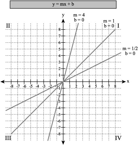
When you set the slope (m) to 1, you multiply the value of the domain (x) by 1, so as you move into quadrant I, for each unit on the x axis, you generate a corresponding and equal unit on the y axis. For example, when the line with slope 1 reaches the dashed graph line for the value of 4 on the x axis, it also reaches the dashed graph line for the value of 4 on the y axis.

The situation changes when you set the slope (m) to 4. When you set the slope to 4, then each unit in a positive direction on the x axis corresponds to a movement of 4 units on the y axis. In the Cartesian plane Figure 6.2 illustrates, you increase the value of the slope until you reach 8, at which point the “rise” of the line has progressed at a rate of 8 units for every 1 unit in the “run” (1, 8). At this point, you are out of room for expansion. Given a larger coordinate system, you could continue to increase the slope indefinitely.

In the same way, when you set the slope to , then for each unit on the x axis, you find only half a unit on the y axis. When the line with a slope of reaches the dashed line for the value of 6 on the x axis, it has climbed only to the value of 3 on the y axis (3, 6). The larger the value of the denominator of the slope, the smaller the rise of the line. For a slope of , for example, when the line reaches the dashed line corresponding to the value of 8 on the x axis, you find that it has climbed only to 1 on the y axis (8, 1).

y-Intercept

As mentioned previously, the constant b in the slope-intercept equation designates the point at which the line crosses the y axis of the Cartesian plane. Figure 6.3 illustrates lines with the same slopes as shown in Figure 6.2. In this instance, however, you change the value of the y-intercept (b). When you assign a value other than 0 to the y-intercept, the line no longer crosses the x axis at its origin. When you set the y-intercept to a positive value, it crosses the y axis above the x axis.

When you set the value of the y-intercept (b) to 4 in Figure 6.3, the line crosses the y axis at 4. When you set it at 2, it crosses the y axis at 2. For the line with a slope of , when you set the y-intercept value (b) to 1, then you shift the line upward by 1, so it crosses at 1. In each chase, changing the y-intercept does not alter the slope of the line. It affects only the position at which the line crosses the y axis.

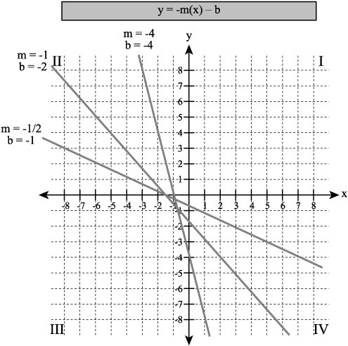
Negative Slopes

As Figure 6.4 shows, when you assign a negative number to the slope value of the slope-intercept equation, you reverse the slope. The slope now slants from the upper left (quadrant II) toward the lower right (quadrant IV). The general relations between values you see with positive slopes continue to apply, however. If you set the slope to –1, then the y value that corresponds to 1 on the x axis becomes –1. If you set the slope to –4, then the y value that corresponds to 1 on the x axis becomes –4. Similarly, for 6 on the x axis, if you set the slope to –, you find that the corresponding value on the y axis is –3. The same applies to the y-intercept values. A value of 2 for the y-intercept causes the line to cross the y axis at 2.

As the lines in quadrant II of Figure 6.4 reveal, when a domain (x) value is negative, multiplying by a negative slope generates a positive range value. As a result, the value of y continues to grow as x becomes more negative. On the other hand, since the values of x are positive, multiplying by a negative slope generates a negative number, so the range values become more negative in quadrant IV as the positive value of x increases.

Negative Shifts

You can define linear equations so that the y-intercept is negative. As Figure 6.5 illustrates, when you combine a negative slope value with a negative y-intercept, the line shifts down on the y axis and slopes downward toward quadrant IV. It no longer passes through quadrant I. When you set the slope to –1 and the y-intercept to –2, then the line crosses the y axis at –2. The value of y when x equals 2 is –4. On the other side of the y axis, when x is equal to –2, y is equal to 0. Multiplying a negative value of x by the negative slope generates a positive value, so the value of y continues to increase as the negative values of x increase.

Exercise Set 6.1 For each line, find the slope and y-intercept. Graph the line. y = 4x + 3 y = –2x – 2 y = –2x + 3 y = 3x – 2 y = –5x + 5 y – 3 = 5 y = x + 5 y = x – 7 y = x y = x + 6