
Varieties of Translation
Translating the curves generated by equations with exponents entails performing operations similar to those you perform with linear equations. On one basic level, translation involves moving the vertex of a parabola along the y axis. To move a vertex along the y axis, you first consider the position of a parabola with its vertex resting on the origin of the Cartesian plane. You can then add values to this position to shift it up or down the y axis.
Parabolas
When you calculate values for a parabola, you use an exponent of an even value. The result is a graph that is symmetrical with respect to the y axis. A parabola crosses the y axis once, so if you employ an equation of the form y = x2 + c, the value of c provides a translation value that is also the value of the y-intercept. As a translation value, the constant c moves the graph up or down the y axis. Figure 10.24 provides a few examples of translation.
Figure 10.24. Add a constant value to shift the graph up and down along the y axis.
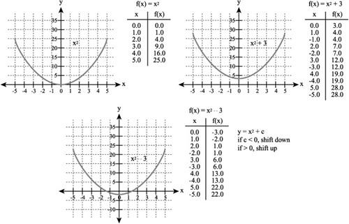
Each parabola shown in Figure 10.24 represents an equation that includes a constant for the y-intercept. In the first use of the equation, you can rewrite it as x2 + 0. When the vertex rests on the coordinates (0,0), the y-intercept value is 0. The other two uses of the equation set the y-intercept at values greater than or less than zero. The first adds 3. The second explicitly subtracts 3.
The generalization then arises that if the value of the y-intercept exceeds 0, then the graph shifts upward. On the other hand, if the value of the y-intercept is less than 0, then the graph shifts downward. When the value of the y-intercept equals 0, then the vertex of the graph rests on the x axis.
To employ Visual Formula to implement a set of non-linear equations that are shifted along the y axis, use these steps (refer to Figure 10.25):
Click the menu item for Value. To position the Value field, click in the upper equation composition area. Type x in the Value field.
Click the Power menu item. Click to place the field for the exponent to the upper right of the Value field. Type 2 in the Exponent field.
Click the Add menu item. Then click to the right of the Value field to position the plus sign.
Now proceed to the lower-right panel and click the Chart for Formula 1 button to generate the graph. As Figure 10.25 illustrates, the vertex of the parabola that results rests above the x axis.
Figure 10.25. Different y-intercept values shift the parabolas up and down the y axis.
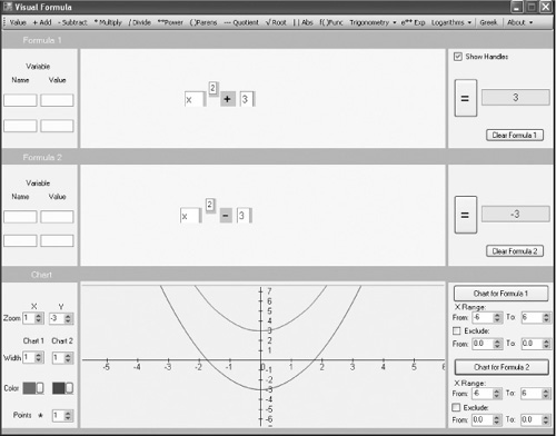
The y-intercept forced the top parabola in Figure 10.25 to shift three units above the x axis. To generate the bottom parabola, perform the following steps:
Click the menu item for Value. Then click in the lower equation composition area to position the Value field. Type x in the Value field.
Click the Power menu item. Position the field for the exponent to the upper right of the Value field. Type 2 in the Power field.
Click the Subtract menu item. To position the minus sign, click to the right of the Value field.
Click Value in the menu. To position the Value field, click after the minus sign. To lower the vertex of the parabola 3 units below the x axis, type 3.
In the Chart panel, set the x axis and y axis Zoom fields to 1 and –3, respectively.
In the lower-right panel, click the Chart for Formula 2 button to generate the graph. As Figure 10.25 illustrates, the vertex of the graph that appears rests three units below the x axis.
Parallel Lines
The general form of the line’s slope-intercept equation is y = mx + b. In this equation, m describes the slope of the equation, and b provides the value of the y-intercept. Given that a set of equations possesses the same slope, if you vary only the value of b, you end up with a set of parallel lines.
Figure 10.26 illustrates the graphs of three lines. The middle line crosses the origin of the Cartesian plane. You could rewrite it as y = x + 0. The other two lines include positive and negative values for the y-intercept. The top line provides a y-intercept of 3. The lower line provides a y-intercept value of –3.
Figure 10.26. The value of the y-intercept raises or lowers the line on the y axis.
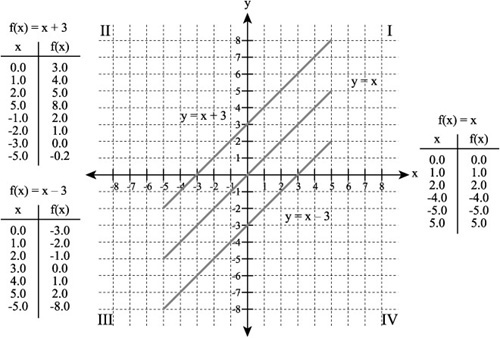
A generalization emerges from the work of these intercepts. If the intercept value is 0, then the line crosses the origin. If it is greater than zero, then the line crosses the y axis above the origin. If it is less than 0, then the line crosses the y axis below the origin. Whatever the y-intercept value, as long as the slopes remain the same, the lines remain parallel.
You can create parallel lines if you set the slope of the line to 1. In this instance, the equation assumes the form y = x + b, for the slope, m, equals 1. To use Visual Formula to generate a set of lines’ slopes set to 1 but y-intercept definitions set at distinct values, follow these steps (refer to Figure 10.27):
Click the menu item for Value. Then click in the upper equation composition area to position the Value field. Type x in the Value field.
Click the Add menu item. Then click to the right of the Value field to position the plus sign.
Now proceed to the lower-right panel, and click the Chart for Formula 1 button to generate the graph. As Figure 10.27 illustrates, the line that results intersects the y axis above the x axis.

In Figure 10.26, you created a line that intercepts the y axis 3 units above the x axis. To create a line that intercepts the y axis 3 units below the x axis, use the following steps:
Click the menu item for Value. Then click in the lower equation composition area to position Value field. Type x in the Value field.
Click the Subtract menu item. Then click to the right of the Value field to position the minus sign.
Click the Value menu item. To position the Value field, click after the minus sign. To set the y-intercept 3 units below the x axis, type 3 in this field.
To generate the graph of the line, in the lower-right panel click the Chart for Formula 2 button. As Figure 10.27 illustrates, the resulting graph crosses the y axis below the x axis.
Odd Exponents and Translations
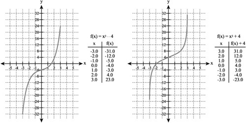
When you work with odd-numbered exponents and do not translate them up or down the y axis, the graphs you generate are symmetrical with respect to the origin of the Cartesian plane. When you change the position of the y-intercept for such equations, the shape of the graph remains the same, but it is no longer symmetrical with respect to the origin. Figure 10.28 illustrates the graphs of equations containing cubed variables. Both equations take the form y = x3 + b. On the right side, the value of b is negative. On the left side, the value of b is positive.
Figure 10.28. The value of the y-intercept moves the graph up or down without distorting it.
To use Visual Formula to create graphs of lines generated by equations that contain variables with odd-numbered exponents, follow these steps (refer to Figure 10.29):
For the first equation (y = x3 + b), click the menu item for Value. Then click in the upper equation composition area to position the Value field. Type x in the Value field.
Click the Power menu item. Then click to the upper right of the Value field to position the Exponent field. After you position the Exponent field, type 3 in it.
Now click the Add menu item and in the equation composition area, click to the right of the Value field to position the plus sign the Add menu item provides.
Click the Value menu item. To position the Value field, click after the plus sign. This is the y-intercept of the equation. Type 4 in the field.
Set the Zoom values to –5.
To generate the graph, locate the lower-right panel and click the Chart for Formula 1 button. As Figure 10.29 reveals, the cubic exponent, combined with the positive value of the y-intercept, causes the graph to cross the y axis above the x axis.
Figure 10.29. The translated results of a function that contains a cube creates a graph that is symmetrical to a line.
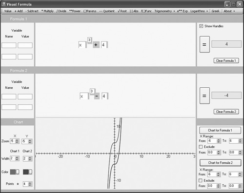
You see the second, lower graph in Figure 10.29. The lower graph crosses the y axis 4 units below the x axis. To create the equation that generates this graph, use the following steps:
Click the menu item for Value. Then click in the lower equation composition area to position Value field. Type x in the Value field.
Click the Power menu item. To position the Exponent field, click to the upper right of the value. After you position the Exponent field, type 3 in it.
Click the Subtract menu item. Then click to the right of the Value field to position the minus sign.
Now click Value in the menu. To position the Value field, click after the minus sign. Type 4 four in the field. This value lowers the vertex of the parabola 4 units below the x axis.
To generate the graph, locate the lower-right panel of Visual Formula and click the Chart for Formula 2 button. As Figure 10.29 illustrates, a second graph appears, lower than the first.
Translating Absolute Values
As previous exercises emphasized, when you plot the solutions to an equation that contains an absolute value, the graph that results is symmetrical with respect to the y axis, and you can shift equations containing absolute values along the y axis. Shifting involves changing the value of the y-intercept. Figure 10.30 illustrates shifting using positive and negative y-intercept values. One graph moves the y-intercept up to 6. The other moves it down to –6.
Figure 10.30. Equations involving absolute values generate graphs that are symmetrical to the y axis.

To use Visual Formula to graph the solutions of equations that shift the graphs of absolute values, follow these steps (refer to Figure 10.31):
For an equation that reads y = |x| + b, work in the top equation composition area. First, click the Abs menu item. Then click in the equation composition area to position the absolute value bars.
Click the Add menu item. To position the plus sign, click to the right of the second absolute value bar.
Select Value from the menu, and then click to place the Value field after the plus sign. This is the y-intercept of the equation. Type 6 in this field.
Now proceed to the lower-right panel of Visual Formula. Locate the X Range fields under the Chart for Formula 1 button. Click the From control and set the value of the field to –10. Click the To control and set the value of the field to 10.

To experiment with the graph of the absolute value figure you see in Figure 10.31, return to the upper equation composition area and change the value of the y-intercept to 4, 5, –4, and –6. The changes you make to the y-intercept value move the graph along the y axis without distorting it.