Secrets of the Ribbon

The Ribbon is the control strip that runs across the top of the Excel window below the window's title bar and any toolbars you've chosen to display. The Ribbon is a control bar that contains multiple tabs, each containing several groups of controls. At any time, the Ribbon displays one tab's contents; to switch to the contents of another tab, you click that tab. As you can see in Figure 1–2, the active tab is a different color than the other tabs, so you can easily pick it out.

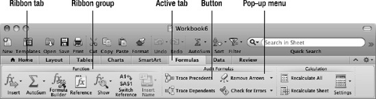
Figure 1–2. The active tab of the Ribbon appears in a different color than the other tabs. Each tab contains groups of controls, such as buttons and pop-up menus.

Understanding How the Ribbon's Tabs Work

Most of the time, the Ribbon displays eight tabs that contain controls for most normal operations in Excel:

• Home. This tab contains controls for cut, copy, and paste; font, alignment, and number formatting; conditional formatting and styles; inserting and deleting rows, columns, and cells; and applying themes.
• Layout. This tab contains controls for manipulating page setup, changing the view, choosing which items to print, and arranging workbook windows.
• Tables. This tab contains controls for working with data tables, which you use for creating databases in Excel.
• Charts. This tab contains controls for inserting charts and sparklines (miniature charts that fit in a single cell), choosing the layout for charts and sparklines, and applying layouts and styles to charts.
• SmartArt. This tab contains controls for inserting and formatting SmartArt graphics.
• Formulas. This tab contains controls for inserting functions, auditing formulas, and controlling how Excel performs calculations.
• Data. This tab contains controls for sorting and filtering data, creating PivotTables and performing what-if analysis, connecting to external data source, validating data, and grouping and outlining worksheets. (Chapter 3 discusses grouping and outlining.)
• Review. This tab contains controls for checking spelling, working with comments, applying protection to a worksheet or workbook, and sharing a workbook.

As well as these standard tabs, the Ribbon contains other tabs that it displays only when you need them. These are sometimes called context-sensitive tabs. For example, when you select a chart, Excel automatically displays the Chart Layout tab and the Format tab (see Figure 1–3).

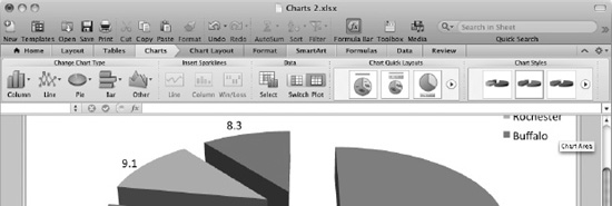
Figure 1–3. The Ribbon displays context-sensitive tabs when you select an object for which tabs are available. Here, the Chart Layout tab and Format tab appear on the Ribbon because a chart is active.

Understanding How the Ribbon's Groups and Controls Work

Chances are you got the hang of using the Ribbon's tabs the first time you used Excel. The groups and controls are a little trickier because they change depending on whether the Excel window is wide enough to display the entire Ribbon.

When the Excel window is wide enough, all the groups appear, and they display their controls—the buttons, pop-up menus, check boxes, and so on—in their most spacious arrangement. For example, the top part of Figure 1–4 shows the rightmost sections of the Layout tab of the Ribbon. All the controls in the Print group and the Window group appear with labels, so you can easily identify each control.

But when there's less space, Excel gradually collapses parts of the Ribbon so as to display as much as possible in the available space. For example, the middle part of Figure 1–4 shows the rightmost sections of the Layout tab again, but this time the labels have disappeared from the Split button, Arrange pop-up menu, Save Layout button, and Freeze Panes pop-up menu. In the Print group, the Fit To label still appears, but Excel has removed the “page(s) wide” and “page(s) tall” labels to save space.

When the window is even narrower, Excel collapses the groups and controls further. In the lower part of Figure 1–4, you can see that the Print group now contains only the Preview button and the Setup button. But you can click the Setup button to display the Print Setup dialog box, in which you can configure all the Print group settings the Ribbon has hidden, not to mention other settings.

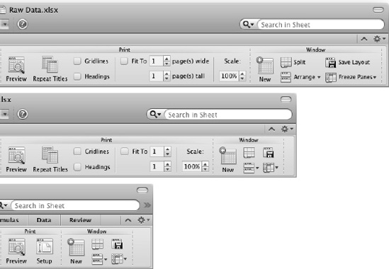
Figure 1–4. As the Excel window becomes narrower, Excel hides first the labels for the less important controls and then the controls themselves, as you can see here with the controls in the Print group and Window group of the Layout tab.

By automatically changing the Ribbon to suit the window width, Excel keeps as many controls as possible at the tip of your mouse. But because labels may not appear, you will sometimes need to display the ScreenTip to identify a control; to display the ScreenTip, hold the mouse pointer over the control for a moment (see Figure 1–5).

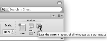
Figure 1–5. When a control's label doesn't appear on the Ribbon, hold the mouse pointer over the control to display a ScreenTip explaining what it does.

Further, because some controls may appear in different places when the Ribbon's whole width isn't displayed, you may sometimes need to hunt for the controls you need. This book assumes that the window is displayed wide enough for you to see all the controls on the Ribbon, but it notes some of the disappearing controls that can cause confusion.

If you can't see a command that's supposed to be there, have a poke around the remaining controls in the group to find where Excel has hidden the control, or to see if one of the controls opens a dialog box that contains the controls. (Or use the menu alternative if there is one.)

Collapsing the Ribbon

When you need more space to work on a worksheet, collapse the Ribbon to just its tab bar (see Figure 1–6) in one of these ways:

• Click the tab that's currently active.
• Click the Collapse Ribbon button (the ^ button) at the right end of the Ribbon.
• Choose View Ribbon from the menu bar (removing the check mark next to the Ribbon item).
• Press Cmd+Option+I.

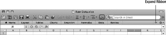
Figure 1–6. Click the Collapse Ribbon button to collapse the Ribbon to just its tabs. Click the Expand Ribbon button (which replaces the Collapse Ribbon button) to expand the Ribbon again.

As you'd guess, you use almost the same moves to display the Ribbon again:

• Click the tab you want to see.
• Click the Expand Ribbon button (the  button) at the right end of the Ribbon.
• Choose View Ribbon from the menu bar.
• Press Cmd+Option+I.