Combination of Laboratory Micro-CT and Micro-XRF on Geological Objects
ABSTRACT: Laboratory micro-CT scanning is a very useful tool in the characterization of geological samples. Due to its ability to visualize different phases and structures in 3D, many characteristics can be derived from the data. However, very limited chemical information on the different phases can be derived by CT. Micro-XRF (µXRF) images this compositional information for a wide range of samples. In µXRF, a 2D grid of fluorescence spectra is collected from the surface of the sample, generating 2D maps of the elemental composition of this surface. By extrapolating the gray values of the µCT data, this information is eventually known in the whole 3D structure.
KEYWORDS: µCT scanning, x-ray fluorescence, element mapping, granite
1. Introduction
Although x-ray micro-CT is a very powerful tool for structural analysis of geological samples, it gives very little information on the chemical composition of the different structures visible in the sample. Since the attenuation coefficient strongly depends on the atomic number of the elements composing the material, an educated guess can be obtained for simple samples. For more complicated samples such as granite or very low concentrations, a more detailed analysis is necessary.
X-ray fluorescence (XRF) captures this information from the surface of a sample. In micro-XRF, the surface is scanned through a focused x-ray beam, and a fluorescence spectrum is measured for each point on a 2D grid. The intensity of the different fluorescence peaks is related to the abundance of the corresponding chemical elements. These peak intensities can then be visualized as elemental maps, showing the relative abundance of each element on the surface.
Although this is similar to what can be done in SEM-EDX, µXRF has some advantages over this technique such as simple sample preparation (Nicolosi et al., 1998), lower detection limits and a less stringent limitation on the size of the sample (Newbury and Davis, 2009). The higher penetration depth of x-ray compared to electrons can be seen both as an advantage and a drawback.
When this information is combined with µCT data, it becomes possible to fully identify the different phases seen in the 3D structure.
2. Experimental setup
To obtain this chemical information, different approaches can be used. For this paper we have focused on XRF-based measurements, as this technique is the most versatile towards sample size, sample type and field of view.
Two different experimental setups were used, each with its advantages and limitations. In the first, the sample under investigation was scanned at the UGCT (Ghent University Center for X-ray Tomography, http://www.ugct.ugent.be) microCT scanners, and afterwards elemental surface maps were recorded with an EDAX Eagle III laboratory µXRF instrument at the XMI (X-ray Microspectroscopy and Imaging, http://www.xmi.ugent.be) research group. This combination offers high accuracy and reliable results, but it requires two separate measurements, implying long measurement times and manual alignment of the resulting data. In a second, more experimental setup, a Canberra X-PIPS™ spectroscopy detector is added to the UGCT µCT scanner, recording XRF spectra from the sample while illuminated for the CT projections. This parallel measurement is less time-consuming, but since the complete sample is illuminated, it has a very low spatial resolution and can only be used to obtain global information on the sample.
Three different samples were used for this research. A Precambrian granite from China (Yellow Rock) was used for identification of the different phases, seen both on the CT data and by visual inspection. A limestone from Maastricht (Netherlands) treated with a silicon-based consolidant at one side was analyzed by µXRF to determine the penetration depth of the consolidant, based on the silicon concentration in the rock. A third sample, a volcanic rock, was analyzed only at the CT scanner, where global information on the composition was obtained with the X-PIPS™.
3. Results
3.1. Yellow rock granite
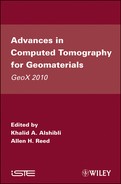
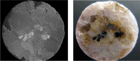
A granite rock consists mainly of quartz, Na-Ca feldspar and K-Na feldspar, with a minor contribution of ferromagnesian phases and some other trace phases. This variety of mineral phases results in a typical heterogeneous look. Visually these phases are hard to distinguish exactly, especially in 3D, because of the optical transparency of some phases. In the 3D rendering of the CT data, the phases show sharp boundaries. The comparison between both can be seen in Figure 1. Except for the high-density features in the middle of the object, there is little resemblance between both.
Figure 1. Comparison between 3D rendering (left) and visual image (right) of the analyzed surface. Total diameter = 8 mm
µXRF measurements (Figure 2) resulted in high silicon concentrations in most of the sample, but different concentrations can be easily distinguished on this map. Note in this respect the very low silicon count rate in the centre of the sample. The elemental map for aluminum is almost binary, showing regions with and without aluminum. A similar result is found for potassium. For the high density region, different concentrations of mainly iron, manganese and titanium can be found.
Figure 2. Element maps for Al, Si, K, Fe, Mn and Ti for the granite surface shown in Figure 1 (map dimensions: 51×200µm by 51×200µm)
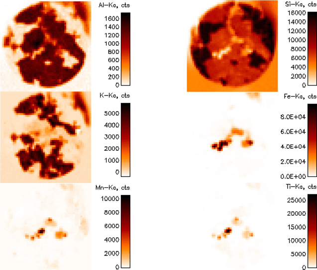
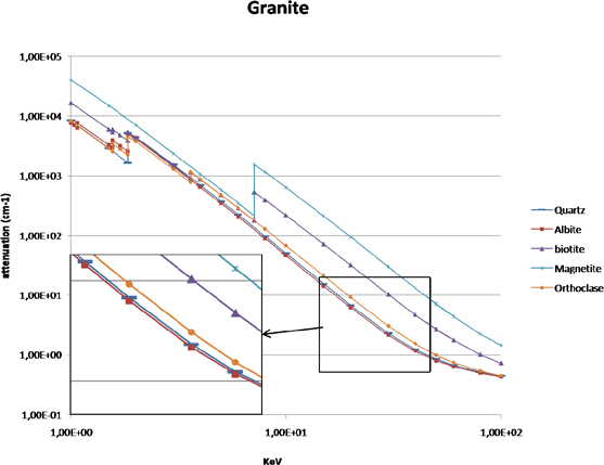
With this information, one can identify the different minerals. The main mineral phases of this granite are biotite (M(Mg,Fe)3(Al,Si)4O10(OH)2), magnetite (Fe3O4), quartz (SiO2), orthoclase (KAlSi3O8) and albite (NaAlSi3O8). Linear attenuation coefficients of these minerals show very similar values for albite and quartz (Figure 3), which explains the identical gray values in the CT data.
Due to the high penetration depth of x-rays, XRF radiation is created in a large part of the sample, especially compared to SEM-EDX. However, the thickness of the measured surface layer is limited by the absorption of the exiting radiation by the material. This can be self-absorption for a homogeneous surface layer, or absorption by a different material. In Figure 2, this latter can be expected around the very intense hotspots of the Fe mapping, where a large spot of lower intensity is seen. This is assumed to be magnetite covered by a thin layer of albite. In Figure 1, this covering can also be seen visually. Based on data extracted from the NIST XCOM photon cross sections database, it can be calculated that the measured Fe-Kα peak intensity (at 6.4 keV) of magnetite covered with 37 µm of albite is about 50% of the measured peak intensity for magnetite at the surface. Although this is a greatly simplified calculation, which ignores all effects such as the focusing of the x-ray beam, it is a good estimate of the thickness of the measured surface layer.
Figure 3. Linear attenuation coefficients of different phases in granite. Region of interest for the CT scans is 30-80 keV
3.2. Maastricht limestone
The Maastricht limestone is a very porous limestone with high concentration of calcite. A block of this material (50×50×50 mm3) was treated with a silicon-based consolidant at one side. The penetration depth of this consolidant material was investigated, as this determines also the quality of the process (Cnudde et al., 2004). To obtain higher CT resolution on this sample, a smaller subsample (8×8×50 mm3) was taken for the analysis. Two CT scans were taken for achieving the highest resolution, one at the treated side of the sample and one at the un-treated side. A difference in porosity is expected between both sides, as pores are filled up by consolidant. A µXRF surface mapping (151×21 pixels, pixel size 200×200µm2, resulting in an area of approx. 30×4 mm2) was measured.
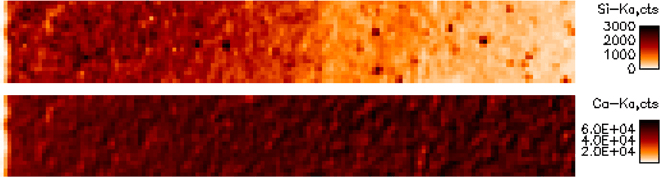
As expected from the CaCO3 bulk composition, the surface map showed very high Ca abundances over the full sample. A much higher Si intensity can be seen at the treated side than inside the sample (Figure 4), showing a consolidant penetration depth of about 15mm.
Figure 4. Si and Ca elemental maps on the treated Maastricht limestone. The treated surface is at the left-hand side. Total area approx. 30×4 mm2
Analysis of the CT data using Morpho+ (Vlassenbroeck et al., 2007) showed indeed a decrease in porosity between the two ends. In the scan of the treated surface, an average porosity of 42.5% was measured, to be compared with 46.2% on the other side. Although these porosities are no absolute figures due to the thresholding, they can be compared since scanning conditions and method of analysis were exactly the same. The consolidant can also be observed on the CT slices as regions of lower density between the grains of the limestone.
The same method was applied on a Bray sandstone. However, since this stone is almost pure quartz, the relatively small consolidant signal could not be distinguished from the intense SiO2 matrix contribution. The porosity measurements reveal a similar effect, with 18.2% porosity at the bulk and 15.1% at the treated surface, indicating the presence of consolidant.
3.3. Volcanic rock sample
A series of scoria and pumice, coming from the area west of the Lac Pavin (lake in Auvergne, France) were scanned and analyzed at UGCT (Vandeputte, 2009). Due to their irregular shape, obtaining a 2D surface map was impossible. An experimental method was applied to these samples. During the CT scan, several XRF spectra were measured using the Canberra X-PIPS™ detector. Since the sample is rotating in a uniform way, angular information on the composition was obtained.
Two great advantages of this technique are the non-destructive nature, and the timesaving caused by the simultaneous measurement. However, the accuracy of the technique is very low. This is mainly due to the total illumination of the sample, which obstructs spatial resolution. This spatial resolution can be achieved by collimation, but this would reduce the measured XRF signal. Another problem is the irregular shape, causing the geometry to change for each angle. It would therefore be necessary to perform a normalization to correct for this. Two straight-forward methods are normalization based on the total background (scatter) counts measured, or based on the tungsten L-lines since no tungsten is expected in the sample, or a combination of both. These methods still need to be tested and verified on phantom samples.
Figure 5. Overview of XRF intensities for some elements found in the analysis, for 6 different angular intervals. Normalization has been performed based on W-Lα intensity
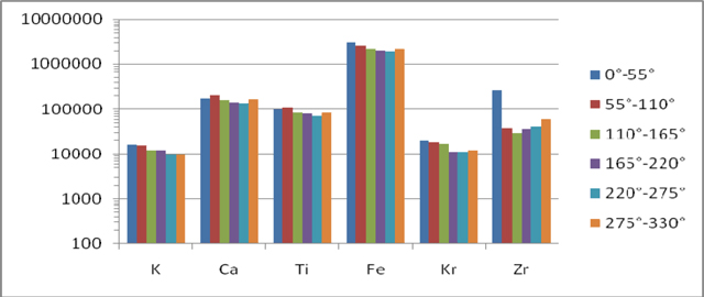
Figure 5 shows the XRF intensities of some elements found in the spectral analysis. Normalization based on tungsten peak intensity has been performed. From this graph, it can be seen that Zr is particularly heterogeneous in the sample, while matrix material such as Ca has a relatively homogeneous distribution. Other detected elements have been left out for clarity. Note that this is only a preliminary result, and the normalization method has to be verified on phantom samples.
4. Conclusion
Combining CT data with µXRF measurements can provide useful information on the 3D structure of the different phases inside complex geological samples such as granite.
µXRF measurements can also be used for the detection of foreign substances in samples, such as consolidant in limestone.
For samples with an irregular shape, a good µXRF surface map can not be obtained. However, XRF measurement during the CT scan can already give information on the sample, although spatial resolution is very poor. This can be improved by a pinhole, but this comes with a reduced countrate. Based on phantom samples, this trade-off will be evaluated. Peak normalization will be tested and refined based on known samples.
5. References
Cnudde, V., Cnudde, J.P., Dupuis, C., Jacobs, P. “X-ray micro-CT used for the localization of water repellents and consolidants inside natural building stones”, Materials Characterization, vol. 53 no. 2-4, 2004, p. 259 – 271.
Newbury, D.E. and Davis, J.M. “Solving the micro-to-macro spatial scale problem with milliprobe x-ray fluorescence/x-ray spectrum imaging”, Proceedings of the SPIE – The International Society for Optical Engineering, Scanning Microscopy 2009, Monterey, CA, USA, 4-7 May 2009, p. 73780P
Nicolosi, J.A, Scruggs, B. and Haschke, M. “Analysis of sub-mm structures in large bulky samples using micro-X-ray-fluorescent spectrometry”, Advances in X-ray Analysis, 1998, 41:227-233
Vandeputte, K. Master’s thesis, Ghent University, Belgium, 2009.
Vlassenbroeck, J., Dierick, M., Masschaele, B., Cnudde, V., Van Hoorebeke, L., Jacobs, P. “Software tools for quantification of X-ray microtomography at the UGCT”, Nuclear Instruments and Methods in Physics Research Section A: Accelerators, Spectrometers, Detectors and Associated Equipment, 2007, 580(1):442-445.