
Micro-Petrophysical Experiments Via Tomography and Simulation
Micro-petrophysical experiments
ABSTRACT. Increasingly, x-ray micro-tomography is being used in the observation and prediction of petrophysical properties. To support this field there is a vital need to have well integrated and parallel research programs in hardware development, structural description and physical property modeling. There is a constant need to validate simulation with physical measurement, and vice versa. Greatly assisting these demands is the ability to perform direct image-based registration in which the tomograms of successively disturbed (dissolved, fractured, cleaned, etc) specimens can be correlated to an original undisturbed state in 3D. In addition, 2D microscopy of prepared sections tie chemical analysis back to the 3D datasets giving a multimodal assessment.
KEYWORDS: quantitative analysis, micro-tomography, visualization, petrophysics
1. Introduction
Over the past 2 decades x-ray tomography has found wide application in the petroleum industry (Withjack, 1988), with particular focus on visualizing potential core damage and the tracking of fluids distribution during flooding experiments. At first, tomography was conducted on the millimetric scale with medical instruments but now micrometric tomography is readily accessible. Ready access to faster computer hardware has provided the opportunity to conduct more complex experiments and the possibility to directly incorporate the 3D tomographic data into modeling/simulation. The increased ease of data collection has not been matched by the improved ability to manage, compare or process this data. Clearly, to take advantage of this “data storm” it is necessary to control the whole data lifecycle, starting with hardware design through to the validation of simulated data. The task is not trivial and must be supported in turn by a holistic view of data and analysis management. In the sections below we will first examine some of the key steps that aid the integration of data on all levels. Finally, several cases studies will be used to illustrate the utility of this approach.
The profile of a tomography facility depends very much on the user-base. The facility described here was specifically assembled to develop the associated hardware to a point where it feeds the highest quality data feasible into a research program in granular and porous materials. Necessarily, there is overlap in skills between experimental, theoretical and computational researchers in the group. In one instance, hardware development is guided by developments in reconstruction theory. Through calibration the comparison of experiment with simulation allows normally inseparable factors to be differentiated.
We will present a range of petrophysical measurements, both virtual and actual, which use tomography as a starting point and matching computer simulation to lab experiments as the goal. Specific systems investigated will include the tracking of acidic dissolution in carbonate sediments, the mapping of residual hydrocarbons after waterflooding into mixed-wet vs. water-wet pore space in reservoir rocks, coincident multi-modal, multiscale imaging of porosity (nm to mm) in carbonate core and monitoring the effects of brine concentration on brine-rock interactions. The key to many of these in situ experiments is the ability to perform direct volume registration in which the tomograms of successively disturbed (dissolved, fractured, cleaned, etc.) specimens can be correlated with each other and with the original undisturbed state in 3D.
2. Work flow
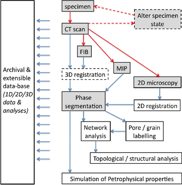
The process to prepare, collect and reconstruct a single high quality tomographic dataset is increasingly straightforward but becomes considerably more challenging once multiple physical analyses or complementary techniques are applied to a specimen. The workflow in Figure 1 illustrates a typical workflow for a specimen analyzed at our facility. The need for calibration and validation at all the stages shown as shaded boxes is paramount if a quantitative view is to be gained. Each of the shaded steps contains intrinsic calibration protocols. It is clear that reconstruction accuracy depends on certain critical CT system parameters, such as magnification and detector calibration, however for many commercial systems these are generally determined only at the time of initial instrument installation. Similarly, electron microscopy involves chemical and detector calibration at a level which is normally insufficient to be reliable for quantitative comparison with tomographic data. A regime of monitoring image quality for 3D and 2D datasets must be an ongoing part of a workflow.
Figure 1. The workflow from experiment through to analysis and simulation. The red arrows illustrate a path that the material specimen takes, the blue arrows refer to data flow The dashed elements show steps that rely on sequential scanning of the same specimen after alteration. The shaded steps require specific calibration against external references. MIP = Mercury Intrusion Porosimetry.
There are a number of ancillary tools, experimental and computer-based which a team relies upon such as, porosity and elemental analyses, visualization and data base management. Data visualization is not, generally speaking, a quantitative tool in its own right but more often than not plays an important role in familiarizing the worker with the dataset. Not to be understated, is the importance data visualization plays in the rapid portrayal of a specimen and accompanying simulation to an uninitiated audience. Tools such as Drishti (http://en.wikipedia.org/wiki/Drishti) help the worker to rapidly understand the relationships between material density, density gradients and spatial distribution. This is particularly useful when other types of data can be superimposed, such as simulation results or 2D micrographs. The shear visual density of tomographic datasets forces the precise identification of material phases to lie in the realm of computational segmentation. Other imaging modalities invariably give either lower spatial resolution or require a 2D section to be taken destructively through the specimen. Comparison of this complementary image data from techniques such as Scanning Electron Microscopy (SEM), with 3D volumetric data greatly enhances material differentiation.
The task of recording the tomographic workflow, from experimental parameters, and related imaging modalities to an historical account of analyses and results requires an extensible data format, in our case, NetCDF (http://en.wikipedia.org/wiki/NetCDF). For the grander task of inter-collating the entire workflow for each experiment in a manner which permits efficient data mining a purpose-built database was designed, Plexus (http://plexus.anu.edu.au/).
3. Material phase segmentation
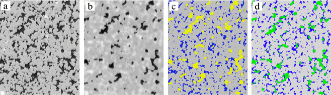
In order to quantitatively calculate physical properties of a specimen from its tomogram, the first step is to classify image voxels according to physical composition. In an x-ray tomogram, the value at each voxel is related to the average x-ray attenuation and depends on the substance located in each voxel. For microtomography, one can assume the material is homogenous within regions much larger than the voxel size. The assumption that voxels are predominantly composed of a single substance will be examined below. Nonetheless, using this assumption reduces the task of determining composition to segmentation: classifying each voxel as a particular component (or phase) according to its associated attenuation value. This task is complicated by the fact that materials are inhomogeneous, they have complex absorption spectra, laboratory-based x-ray sources are strongly polychromatic, and images have noise. Although segmentation is inherently imperfect at component boundaries – where voxels may be composed of several substances – it nonetheless represents the best starting point for quantitative analysis. Once identified, each component is assigned material properties using a priori specimen knowledge, sometimes refined with experimental measurements. Prior to segmentation, we have found that image quality can be significantly improved by the application of an edge-preserving de-noising filter, and that best results are obtained with the 3D anisotropic diffusion filter (Perona, 1990), particularly the hybrid method of Frangakis (Frangakis, 2001). To perform the segmentation itself, we have found that classifying voxels purely according to their local intensity values (i.e. thresholding by intensity) is sufficient only for very high quality images containing two substances. Therefore, non-local and gradient information needs to be incorporated into the segmentation process. There are many published image segmentation techniques and invariably most have the same basic principle: identify seed regions, grow the seed regions based on some rules, and finally terminate at a suitable point. To analyze large tomograms routinely, segmentation must be computationally efficient and allow for data-parallel execution. We have developed a region-growing algorithm that uses the fast-marching method (Sethian, 1996) to achieve a good compromise between segmentation quality and computational efficiency (Sheppard, 2004). This algorithm cannot automatically segment a tomogram; on the contrary, some user skill is required and there tends to be some uncertainty in the outcome. To identify multiple components, the algorithm is applied repeatedly by masking all previously identified components. To demonstrate the technique a two-phase segmentation is shown in Figure 2. Figure 3 demonstrates one of the measures used to check the quality of a segmentation. A simulation of a non-wetting fluid (“mercury”) intrusion is performed on the segmented image and compared against a lab-based MIP measurement on the actual specimen scanned. Although this is a destructive measurement, half the core may be preserved for other analyses. If the simulated intrusion data correlates well with the laboratory intrusion data then we can be confident that the segmented image contains an accurate representation of the pore-space of the specimen. The segmented image is the first stage of processing for many subsequent petrophysical simulations, so it is critical that the MIP experiment validates the segmentation in order to be confident in the subsequent analyses.
Figure 2. A sub-region of a slice from a phase-contrast tomogram of wood, with a voxel size of 700 nm. The experimental data (a), filtered with anisotropic diffusion (b), and an initial threshold is chosen to identify seed regions for the segmentation (c). Blue is the void phase seed and red is grain phase seed. The final segmentation (d) is overlaid on the tomogram; regions of wood phase have been colored green. Adapted from Sakellariou, 2007.
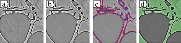
Figure 3. (a) A 500 µm wide subset of a dolomite, and (b) the corresponding 2-phase segmentation. (c) A plot of simulated vs. measured MIP on same specimen scanned
4. Registration
A range of 3D image registration techniques have been developed to extend the capabilities of x-ray micro-CT and to allow the calibration of micro-CT data to other microscopic techniques. In contrast to the alignment of 2D images, for which many tools are publicly available, registration of very large 3D images, for which distributed-memory parallel algorithms are required, pose a considerable challenge. As we are not aware of available software which is capable of accomplishing this task the group has implemented registration techniques (Latham, 2008) which combine a low resolution exhaustive search plus a multi-start, multi-resolution local optimization to achieve accurate spatial alignment of an image pair. Registration of a 2D micrograph with a tomogram (Figure 4) takes typically 1 hour on 64 CPUs, whereas a 3D-to-3D registration takes only about 2 hours on the same number of CPUs (SGI Altix BX2 system). The chief requirement is for significant distributed memory, over 100GB being required for the processing of 20483 datasets.
Figure 4. An illustration of the 2D to 3D registration result. The routine orients any arbitrary slice back into the original containing volume. The linearity of the 2D section must be as well matched to the tomogram as possible. This means better than 1 part in 1000 linearity. The process of registration is contingent on good calibration of both tomogram and micrograph.
The ability to accurately align micro-CT images with images generated from other modalities provides diverse capabilities and the potential to enhance the information present in the micro-CT image. The images in Figure 5 show 2D scanning electron microscopy (SEM) images of polished thin sections extracted from plugs previously imaged by x-ray micro-CT. SEM imaging generates submicron resolution images, and can even provide detailed mineralogical maps through energy dispersive x-ray spectroscopy. Accurate registration of the 2D microscopic image within the 3D image volume increases the potential for mapping x-ray gray-levels to mineral phases, reveals information about features too fine for x-ray micro-CT and provides an invaluable quality control on the 3D image data.
To the eye, 2D micrographs seem undistorted, however to register against a 3D dataset the micrograph must be corrected for non-linearities to better than 1 part in a 1000. SEM images can contain distortions of a few percent, optical micrographs can be worse. Tomograms, by design have undistorted cubic elements (voxels) and, if the x-ray optics have been calibrated appropriately, provide a distortion free cubic grid. In Figure 5 we have also registered an optical thin section of the same slice (again warp corrected). Although polarizing information is difficult to incorporate into a 3D dataset it provides an instant visual key for a trained mineralogist. The advantage here is that a specialist can adapt their intuition for making 3D inferences from a tried and tested 2D methodology.
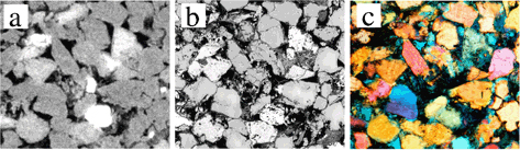
Figure 5. (a) A small region from a tomographic section (˜1 mm wide), (b) the corresponding registered SEM from a polished thin section of the same region, (c) the optical micrograph from the same thin section. All micrographs require linear calibration against an appropriate standard.
Another application of registration is the alignment of tomographic datasets acquired at different resolutions. Figure 6 illustrates the difficulty in considering the multi-scale heterogeneity in carbonate reservoirs. Accurate spatial alignment provides the ability to reconcile differences in physical porosity measurements against computationally derived values from segmentation. In Figure 7 a tomogram of a 25 mm carbonate core was generated with 15 micron voxel size. Subsequently, a 5mm core was drilled from the 25 mm core and scanned with a 5 micron voxel size.
The higher resolution tomogram was then registered with the lower resolution tomogram. The accurate alignment of the two images then allows one to more easily transfer (upscale) the high-resolution porosity data to the larger-scale, or lower resolution, tomogram.
Figure 6. A cross-section through a 44 mm carbonate core with a tomogram from the 5 mm core physically sub-sampled from the region shown. This result is that the resolution is increased by almost a factor of 10. A quantitative measure of the error in porosity can be made by considering these multiscale measurements.
Figure 7. (a) A 15 mm wide sub-set from a tomogram of a 40 mm limestone core (25 micron voxels. The higher resolution inset is shown overlain centrally and is the corresponding slice from the 5 mm core physically sub-sampled from the 40 mm core, and re-scanned. (b) and (c) show registered slices from the 40 mm and 5 mm cores, respectively.
Figure 8. (a) A 1 mm wide sub-set from a tomographic slice of a carbonate. (b) shows four ranges in apparent porosity from solid (blue), light and dark green (micro-porous, sub-voxel resolution) to macro-pore (red, resolved in the tomogram). (c) The corresponding registered polished section from SEM, with (d) illustrating the levels of micro-porosity not assessed in the tomogram. The plot left shows porosity as a function of percentage of voxel filled. The error bars are given by the segmentation of the SEM.
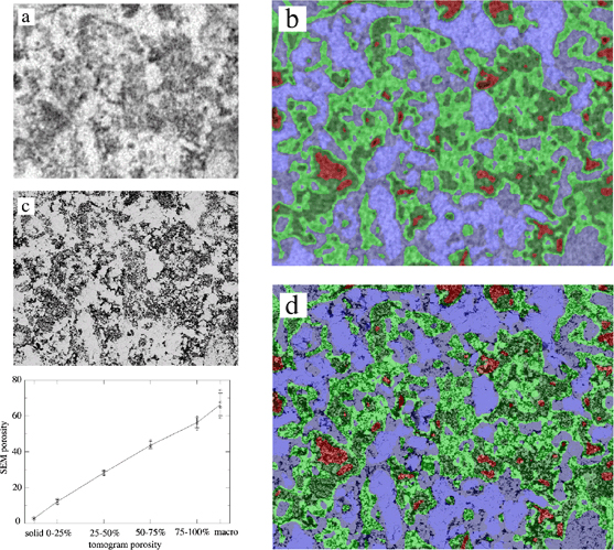
In Figure 8 a study is shown demonstrating a situation where the gray values of the tomogram voxels indicate a partial volume, that is, neither fully pore nor fully solid. This is a typical occurrence in specimens where pore sizes are much smaller than the actual voxel size. In the mono-mineralic system shown, it allows porosity to be calibrated based on gray value. For multi-mineralic systems ambiguities with mineral density and porosity can make this approach very challenging. The opportunity that registration with SEM allows is to validate the choice of effective porosity against apparent 2D porosity. In Figure 8 the registered SEM is used as a mask to define the solid phase so thereby adding certainty to a calibration of effective porosity versus voxel intensity.
5. Case studies
In this section we rely on the registration process to quantitatively incorporate other imaging data and to track the micro-structural changes that occur upon dissolution or fluid ingress. The following classes of studies aim to illustrate the importance of data quality both as acquired from tomography and other modalities. For ease of presentation all cases show only small 2D subsets, but all comments have been derived from analysis on the original 3D datasets.
Sub-resolution porosity: Porosity which is below the imaging resolution continues to challenge tomographic modeling, particularly for multi-mineralic systems such as clay-rich siliclastics. Figure 9 shows how important the integration of other imaging modalities can be for tomography-based simulation. Based on CT data alone only a small proportion of the clay phase is correctly identified. Much of the pore-filling material shows too little contrast to be usefully segmented as clay. Comparison with the registered SEM “calibrates” the selection of segmentation parameters and substantially more clay is identified. At this point the simulation of permeability more closely matches the lab-based whole-core measurements. It is highly instructive to see that, apart from the change in porosity, the electrical conductivity is not very sensitive to the refined segmentation.
Fluid mapping and wettability: the migration of fluid, particularly immiscible fluids such as oil, water and gas on the scale where surface tension dominates the fluid distribution is the chief domain for the geological application of micro-tomography today. To track fluid interfaces at the pore-scale is a major technical challenge. Here we look at addressing this challenge by imaging specimens in different saturation states, using registration to accurately align the tomographic images and subsequently subtracting the aligned images to analyse the fluid distributions. Figure 10 illustrates an initially dry, siliclastic which undergoes two sequential floods with water. The registration is so effective in distinguishing liquid from gas that a minimum of X-ray contrasting medium is needed in the fluid phase, improving overall clarity of menisci and thin films. In the experiment shown in Figure 11 a water solution is allowed to spontaneously imbibe into a dry 5mm core and allow us to equilibrate for 24 hours, Figure 11(b). The trapped gas phase is clearly evident from the image in Fig 11(c). The trapped gas phase saturation is 31%. Imbibition is complex and imaging the resulting pore-scale distribution of fluids can assist in improving our understanding and modeling of the process. The imbibition of a wetting fluid into a porous media is influenced by rate, heterogeneity of the pore space and local pore geometry (Morrow, 1985), which can lead to a wide variety of wetting patterns including site invasion percolation, cluster growth and flat frontal advance (Lenormand, 1984; Blunt, 1995).
Figure 9. (a) A 200 µm wide sub-set of a 5mm core of a clay-rich siliclastic rock showing a “naïve” segmentation based on the tomogram alone. Black represents the grain phase, gray the clay phase and white the pore space. (b) The registered SEM of the same region. (c) A refined segmentation based on the SEM. The top plot shows the effect both on estimated porosity and simulated conductivity for naïve and refined segmentations. The conductivity simulation is finite element based and assumes the presence of a clay phase halves the conductance. Surface conductivity is ignored. Permeability was simulated on sub-volumes of 3603 voxels, and run in three orthogonal directions. The lower plot shows a marked change when clays are more realistically considered. In this case the clay phase is assumed to be essentially non-permeable. The lab-based measurement of permeability on the whole 50 mm core found 0.009 D, consistent with the SEM-informed segmentation.
Figure 10. (a) A 500 µm wide tomographic subset of a dry siliclastic, followed by successive water floods (b), (c). (d), (e) show the level of detail possible in menisci. The next task is to computationally extract interfacial curvatures on the entire dataset
Figure 11. (a) A 600 µm wide tomographic subset of a dry sucrosic dolomite; (b) registered slice after spontaneous imbibition with 0.1M CsI solution; (c) phase separation of pore space allows separation of water (blue) and residual gas (yellow) in 3D. (d) shows the distribution of the trapped phase (green) based on an ordinary percolation simulation in 3D image having the same water saturation as observed experimentally (Kumar, 2009).
Notwithstanding the many complexities, the imaged saturation distributions shown in Figure 11(c) show that the trapped gas phase is concentrated in the largest pores. This suggests that a simple percolation type mechanism may be relevant in describing the process (Wilkinson, 1984). In a percolation-based model of an imbibition displacement the residual (trapped) gas saturation is formed when the displaced fluid (gas) stops percolating or becomes disconnected. This ordinary percolation threshold is easily determined on the 3D image data by incrementally removing spheres in the covering radius map from smallest to largest and tracking when the sphere map first disconnects across the entire core, Figure 11(d).
Figure 12. A 800 µm wide slice from a siliclastic showing dolomitic and anhydrite cement, before (a) and after (b) flushing with low salinity brine (10 milliMolar range). Both tomograms have been registered and 3-phase segmented (black is the pore space, gray is the quartz phase, and white the dolomitic/anhydrite cement phase). CT does not distinguish the different cements well in this case. The red dots in (a) indicate regions where material has mobilized or dissolved.
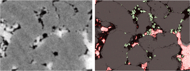
Particulate migration: In a geological context, mineral solubility plays a major role in fluid permeability. As part of a broader study into the effects of salinity of the connate brine on clay migration, Figure 12 shows how single dolomite particles can be mobilized with a drop in brine salinity. The registration of the mineralogical map from SEM, Figure 13, with the tomogram implicates the role of sulfate in the surface conversion of dolomite into anhydrite. This leads to the dislodgement of the dolomite which is then caught by the fluid flow (Lebedeva, 2009).
Figure 13. A 300 µm wide tomographic slice from the siliclastic above registered with a mineralogical map from SEM for dolomite (green) and anhydrite (red). Note that the dolomitic phase on the left is often poorly distinguished from the quartz phase owning to small size. Without registration the difference between surface roughness and a distinctly different phase can be difficult to resolve.
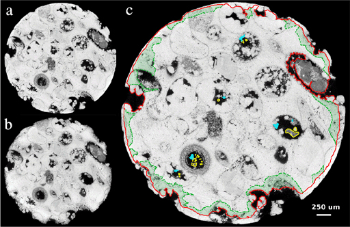
Reactive Fluids: pore structures of rocks can be strongly altered when subject to reactive fluids. For example, the acid dissolution of carbonates leads to a wide range of alteration of pore morphologies; due to the complexity of the pore structures, experiments are necessary to identify the controlling mechanisms of alteration. Micro-CT experiments coupled with 3D registration allow one to probe alteration at the pore scale. A simple reactive experiment was undertaken; a limestone core was vacuum saturated in a bath of CO2 saturated water at 10 atm for 96 hours. Imaging was undertaken before and after the saturation experiment. Image registration enabled us to perfectly align the two images and locally mapping the evolution of the porous microstructure of the carbonate during dissolution/precipitation (Figure 14). The dissolution was mapped despite the sample being moved from the beamline for the 96 hour experiment. A number of longer-term experiments can be undertaken using the registration process rather than having to dedicate an entire CT beamline to a slow process.
Figure 14. Slices from two registered tomograms of a 5 mm diameter oolitic carbonate core exposed to carbonic acid (10 atm CO2 for 96 hours). (a) The initial state, and (b) after dissolution. (c) The red line superimposed on the initial state corresponds to the new boundary after dissolution and the shared green area shows the consequential increase in porosity of the microporous regions. Particles that have been displaced are marked with a yellow line, while particles that are a result of reprecipitation have been indicated with blue.
Mechanical modeling: The morphology of fractured porous media is very complex and involves heterogeneities at several length scales. Analysis of fractures as with sub-resolution porosity relies upon an accurate determination of X-ray optical and reconstruction parameters. The blurring in tomographic data when these parameters are not well defined will readily cause loss of feature definition, but critically loss of phase (fracture) connectivity.
Finite Element Modeling (FEM) is a numerical technique which can be used for solving static elastic equations over a discretized volume and we can simulate the elastic deformation of porous materials and calculate the acoustic response of arbitrary complex media (within resolution limits). More often than not, the computed results are in good agreement with the experiments (Roberts, 2002; Arns, 2002, Gerchka, 2006). Bohn and Garboczi (Bohn, 2003) present a comprehensive description of the FEM’s numerical implementation as applied to 3D digitized images, using a conjugate-gradient algorithm to solve the discretized set of the equations. Although we can use the FEM to determine the numerical solution of any partial differential equation, we consider only the equation of linear elasticity here. Figure 15 shows a 2D slice of a real 3D-fractured medium and the analytical approximation for estimating its properties. For the actual calculations on the fractured samples, we assume that the sample is dry and assign phase moduli of dolomite to the solid phase (K = 69.4 GPa and G = 51.6 GPa). Figure 15 (c),(d),(e) shows slices through the displacement vector fields for three component fields and the fractured sample after the energy is minimized. These results show that displacements on the fracture have been reflected in other directions, indicating that they occurred because of the fracture (which induced a shear-like effect).
Figure 15. (a) A single slice through the fractured sample after anisotropic filtering, (b) the corresponding segmented dataset. (c, d, e) show unit displacements in the three orthogonal directions (see Madadi, 2009 for details)
6. Conclusions
While the estimation of micro-petrophysical properties in 3D still provides enormous opportunities much of the future utility of micro-CT lies in the ability to quantitatively correlate other measurements with this technique, and over a greater range of length scales. Due to the need for up-scaling micro-CT both mineralogy and material moduli mapping will receive attention in the near future. Clearly the management of hydrocarbon reserves is one area to benefit from micro-CT, but studies on regolith and groundwater, mineralization and hydrothermal synthesis, and microfossil identification are just a few to see the benefits of quantitative 3D imaging.
7. Acknowledgements
The authors acknowledge the member companies of the Digital Core Consortium for providing funding support and the Australian Partnership for Advanced Computation for supplying computing resources. We thank also the Australian Research Council for ongoing research support.
8. References
Arns, C.H. et al., “Computation of Linear Elastic Properties from Microtomographic Images: Methodology and Agreement Theory and Experiment,” Geophysics, vol. 67, no. 5, 2002, pp. 1396–1405.
Blunt, M.J. and Scher, H., “Pore level modeling of wetting”, Phys. Rev. E, 52, 6387-6403 (1995)
Bohn, R.B. and Garboczi, E.J. User Manual for Finite Element Difference Programs: A Parallel Version of NIST IR 6269, tech. report 6997, US Nat’l Inst. Standards and Tech., 2003.
Frangakis, AS, Stoschek, A, Hegerl, R. “Wavelet transform filtering and nonlinear anisotropic diffusion assessed for signal reconstruction performance on multidimensional biomedical data”, IEEE Trans. Biomed. Eng. 48, 213 (2001)
Gerchka, V. and Kachanov, M. “Effective Elasticity of Rocks with Closely Spaced and Intersecting Cracks,” Geophysics, vol. 71, no. 3, 2006, pp. D85–D91.
Kumar M, Senden TJ, Knackstedt MA, Latham SJ, Pinczewski, V, Sok RM, Sheppard AP and Turner ML. “Imaging of Pore Scale Distribution of Fluids and Wettability”, Petrophysics, 50(4) 311-321 (2009)
Latham, S.J., Varslot, T. and Sheppard, A.P. “Automated registration for augmenting micro-CT 3D images”, in Proc. 14th Biennial Computational Techniques and Applications Conf, J. ANZIAM, vol.50, pp. C534--C548, 2008.
Lebedeva, E., Senden, TJ, Knackstedt, M.A and Morrow, N. “Improved Oil Recovery From Tensleep Sandstone – Studies of Brine-Rock Interactions by Micro-CT and AFM.” 15th European Symposium on Improved Oil Recovery, Paris 29 April 2009
Lenormand, R. and Zarcone, C., “Role of Roughness and edges during imbibition in square capillaries”, SPE 13264, Presented at 59th Annual Technical Conference, Houston, 1984.
Madadi, M; Jones, AC; Arns, CH, and Knackstedt, MA. “3D Imaging and Simulation of Elastic Properties of Porous Materials”, Computing in Science & Engineering, 11(4), 65-80, 2009.
Morrow, N.R.: “A Review of the Effects of Initial Saturation, Pore Structure, and Wettabilityon Oil Recovery by Waterflooding,” Proc. North Sea Oil and Gas Reservoirs, Trondheim (Dec. 2-4, 1985) Graham and Trotman, Ltd., London,, 179-91 1987.
Perona, P., and Malik, J, “Scale-space and edge-detection using anisotropic diffusion” IEEE Trans. Pattern Anal. Machine Intell. 12, 629 (1990)
Roberts, A.P. and Garboczi, E.J. “Computation of the Linear Elastic Properties of Random Porous Materials with a Wide Variety of Microstructures,” Proc. Royal Soc. London, vol. 458, no. 2021, 2002, pp. 1033–1054.
Sakellariou A, Arns CH, Sheppard AP, Sok RM, Averdunk H, Limaye A, Jones AC, Senden TJ and Knackstedt, MA. “Developing a virtual materials laboratory.” Materials Today, 10, 44-51 (2007)
Sethian, J. A., “A fast marching level set method for monotonically advancing fronts”, Proc. Natl. Acad. Sci. USA (1996) 93, 1591
Sheppard AP, Sok RM, and Averdunk H “Techniques for image enhancement and segmentation of tomographic images of porous materials”, Physica A (339), 145-151 (2004)
Wilkinson, D., (1984), “Percolation in immiscible displacement”, Phys. Rev. A, 34, 1380-1391.
Withjack, E. “Computed tomography for rock-property determination and fluid flow visualization.” SPE Formation Evaluation, 696–704, (1988).