
Factor analysis can be thought of as an extension to principal components. Here, we are interested in identifying the underlying factors that might explain a large number of variables. By finding the correlations between a group of variables, we look to find the underlying factors that describe them. The difference between the two techniques is that we are only interested in the correlations of the variables in PCA. Here, in factor analysis, we want to find the underlying factors that are not being described in the data currently. As such, rotations on the factors can be used to closely align the factors with structure in the variables.
The data has been collected from different automobile manufacturers. The variables look at weights of vehicles, fuel efficiency, engine power, capacity, and CO2 emissions.
We will use factor analysis to try and understand the underlying factors in the study. First, we try and identify the number of factors involved, and then we evaluate the study. Finally, we step through different methods and rotations to check for a suitable alignment between the factors and the component variables.
The following steps will help us identify the underlying factors in the jobs dataset:
- Open the
mpg.MTWworksheet. - Go to Stat, click on Multivariate, and select Factor Analysis.
- Enter
CO2,Cylinders,Weight,Combined mpg,Max hp, andCapacityinto the Variables: section. - Select the Graphs… button and select Scree plot.
- Click on OK in each dialog box.
- Check the results in the scree plot and the session window to assess the number of factors, as shown in the following screenshots:
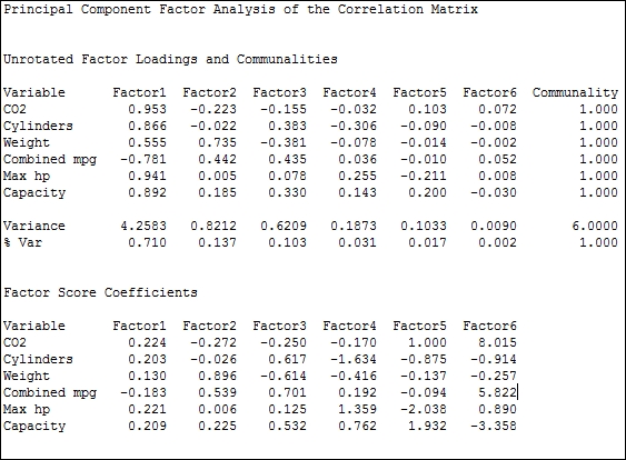
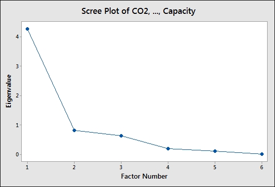
- Here, the results indicate that factors 1 and 2 account for a majority of the variation, factors 3 and 4 account for a similar amount, and the components beyond factor 4 are small.
- Next, we should assess how useful the factors are likely to be. The loadings for factor 1 have high values across most factors and pay particular attention to high
CO2andMax hpvalues, with a strong negative combined mpg. - Assess the model with only the first two factors by returning to the last dialog box by pressing Ctrl + E.
- Enter
2in the Number of factors to extract: section. Click on the Graphs… button and select Loading plot. - Click on OK to generate the loading plot for the first two factors.
- Next, we will assess the model with a rotation. Do we see the same structure using an orthogonal rotation? Press Ctrl + E to return to the last dialog box.
- Change the type of rotation to Varimax.
- Click on OK.
- Compare the loading plot from the varimax rotation to the original loading plot. The same structure should be observed with a rotation between the two factors.
- Next, compare the results from the Maximum likelihood and Varimax rotation. Press Ctrl + E to return to the last dialog box and select the option for Maximum likelihood. Click on OK.
- Compare the loading plots. All loading plots show a similar structure, but with our variables aligned differently to the factors across each rotation and method. The loading plot from the principal components study, using the varimax rotation, may be desirable as PC1 is closely tied to
Combined Mpg, with PC2 showing a strong association withWeight; the factors associated withCapacity,cylinders,hp, andCO2tend to the upper-right corner of the chart. - Press Ctrl + E to return to the last dialog box, select Principal components for Method of Extraction, and Varimax for Type of Rotation.
- Click on the Graphs… button and select Score plot and Biplot to study the results.
- Click on OK in each dialog box.
The steps run through several steps to iteratively compare the factor analysis. The strategy of checking different fitting methods and rotations to settle on the most suitable technique is discussed in "Applied Multivariate Statistical Analysis 5th Edition",Richard A. Johnson and Dean W. Wichern, Prentice Hall, page 517.
The method and type of rotation is probably a less crucial decision, but one that can be useful in separating the loading of variables into the different factors rather than having two factors that are a mix of many component variables.
The strategy, as discussed by Johnson and Wichern in brief, is as follows:
- Perform an analysis of a principal component.
- Try a varimax rotation.
- Perform maximum likelihood factor analysis and try a varimax rotation.
- Compare the solutions to check whether the loadings are grouped together in a similar manner.
- Repeat the previous steps for a different set of factors.
In this example, we will get similar groups of loadings with both fitting methods and rotations. The loadings will be different with each rotation, but they group in a similar way; we can observe this from the loading plot.
The suggestion that the principal components method with Varimax rotation is suitable for this data comes from the line along factor 1 and 2 in the loading plot, as shown in the following figure:
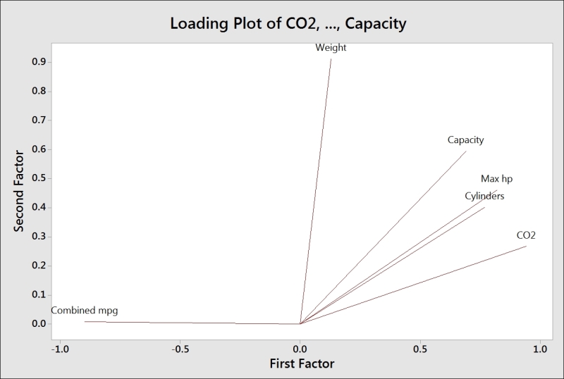
Factor 1 appears to be associated with fuel efficiency versus power and factor 2 with vehicle weight.
Minitab offers Equimax, Varimax, Quartimax rotations, and Orthomax, where the rotation gamma can be chosen by the user.
The storage option allow us to store loadings, coefficients, scores, and matrices. Stored loadings can be used to predict factor scores of new data by entering the stored loadings into the loadings section of the initial solution within options.