
Logistic regression models allow us to fit a regression model to categorical data. Here, we will look at the survival rates of passengers on the Titanic. This data is binomial in that we list the survivors or casualties of the disaster.
We will initially recode the Survival columns to state 1 as survived and 0 as casualty. Then, we study the effects of age, class, and gender on the chances of survival. This isn't essential but can be a useful aid to the interpretation of the results.
The final steps will store the event probability calculated from the fitted model to plot the results in a scatterplot.
The data is contained in test format at the StatSci website. The direct link to the Titanic data is as follows:
http://www.statsci.org/data/general/titanic.txt
The data will copy and paste directly into Minitab. The data columns are listed as Passenger class, Age, Gender, and Survival.
Do make sure that you check the dataset, as a couple of passenger details are shuffled into the wrong columns; for example, rows 296 and 307 need to be corrected manually.
Not all the passengers' ages are listed in this dataset and it is possible to find a listing of this data in other formats with a quick web search.
The Titanic data is available in different formats; performing a search on the Internet will reveal other datasets.
The data at the American statistical association lists passengers as child or adult rather than listing them by age.
The following steps recode the results from numeric values to categorical ones. Then, we fit a binary logistic regression to find how the age, gender, and class affected survival chances. We will then use factorial plots to visualize the fitted model.
- Navigate to Data | Code and select Numeric to Text….
- Enter
Survivedinto the Code data from columns: and the Store coded data in columns: sections. - Enter the original values and the new values as shown in the following screenshot:
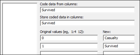
- Click on OK.
- Navigate to Stat | Regression | Binary logistic Regression and select Fit Binary Logistic Regression.
- Enter
Survivedin the Response: section, then enterAgein the Continuous predictors: section, andPClassandSexas Categorical predictors:, as shown in the following screenshot: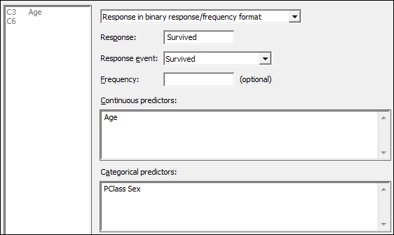
- Select the Model… button and highlight
Age,PClass, andSexin the Predictors: section; in the Interactions through order: section, enter2, then click on the Add button. Click on OK in each dialog box. - Return to the session window and check the results, as shown in the following screenshot.
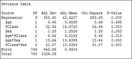
- Use the regression table to look for interactions with a P-value above 0.05, or the Chi-square for interactions with low values.
- As all interactions are significant, we will not reduce the model. To produce diagnostic plots, return to the last dialog box by pressing Ctrl+E.
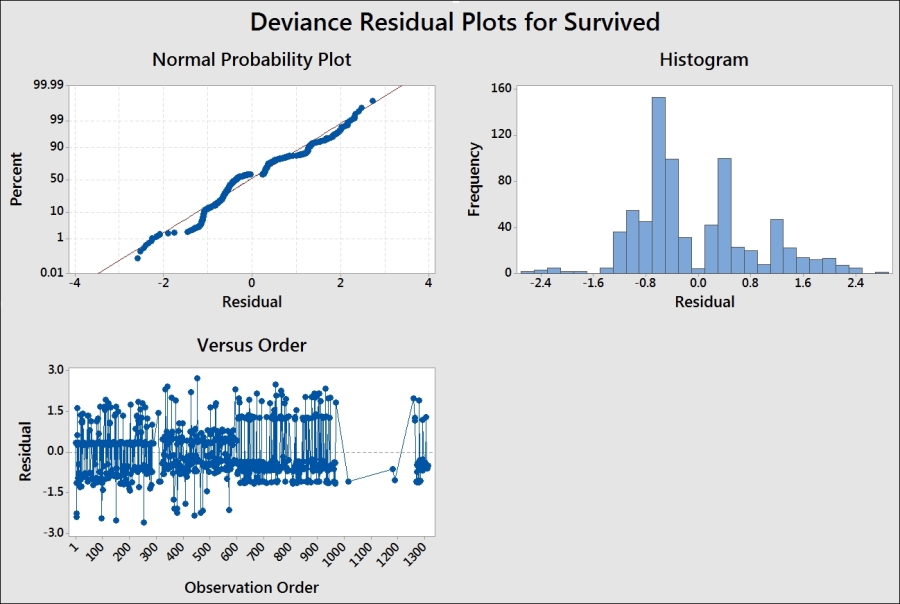
- Click the Graphs… button and select the Three in one residuals. Click on OK in each dialog box.
- To plot the calculated event probabilities, we will use the factor plots. Navigate to Stat | Regression | Binary logistic Regression and select Factorial Plots….
- Move
Agefrom the Available factors: section to the Selected: section by double-clicking onAge. Then click on OK.
The code tool used in steps 1 to 4 works in a way that is similar to an IF statement in the calculator. Although we cannot use this to create a formula in the worksheet, it is a very visual way to recode the data. Ranges of numbers can be coded using a colon as the range separator. For example, 1:10 would specify a range from 1 to 10.
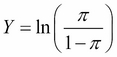
By default, the Binary logistic regression model uses a logit transform with a probability of 0 to 1. The regression is then fitted to the logit transform, which is shown as follows:
Normit and Gompit transformations are also available to be selected from options within Binary Logistic Regression. The Normit transformation uses the inverse CDF of the standard normal distribution to map the probability. For example, a result at +2.326 from 0 has a 99 percent probability of occurring and -2.326 from 0 has a 1 percent probability of occurring.
The Gompit or log model is useful in growth models of biological data as the curve of the function is not symmetric like the Logit or Normit functions.
Minitab has picked the event for the regression model as Survived. The model then calculates the probability of survival. The event is indicated at the start of the analysis. The default event is picked reverse alphabetically. We can change Response event: from the main dialog box to Fit Binary Logistic Regression. This drop down can be used to change between the two possible outcomes.
The Coding… options allow us to choose the reference level of the categorical predictors. Also, here we can change the increment used in calculating the odds ratios for the continuous predictors.
Minitab provides residual plots for either Pearson or Deviance residuals. The residuals can be used to check for outliers or patterns over time in the results, as shown in the following example:
Factorial plots are used to help visualize the result of the logistic regression. Main effects and interaction plots of the fitted probabilities are generated for the three sets of interactions, as shown in the following screenshot:
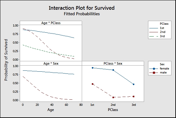
The results show some dramatic interactions between the three predictors used in the model.
We can also generate predicted probabilities with confidence intervals and prediction intervals from the Predict… tool. This has the same options as the predict tool for Regression and Poisson regression.
The Fit Binary Logistic Regression tool can also run a stepwise analysis for us. The options are the same as Fit Regression Model….
- The Coding a numeric column to text values recipe in Chapter 1, Worksheet, Data Management, and the Calculator