
Frequently, we obtain data that does not want to easily fit any distribution or any transformation. The key to using this data is often to understand the reasons for the data not fitting a distribution.
We can find many reasons for not fitting a distribution and the strategies for running a capability analysis can be varied, depending on the cause. For more on some of the issues that we should be careful of when declaring that our data is not normally distributed, see the Capability analysis for nonnormal distributions recipe.
The very first step in any analysis of data that is not normally distributed should be to understand why the data appears as it does.
This recipe explores several issues that may occur in data. This looks at a processing time example. Such data has the lower boundary at 0; this can give us a distribution skewed to the right. The other issue is that of discrete intervals in the data; the measurement system is not truly continuous for these.
Here, we will look at using the wait time data as they were used in the nonnormal examples earlier. This dataset contains wait times at the A&E department of a hospital across one day. Column one contains the data reported in one-minute intervals and column two contains the same data but rounded to the nearest five minutes.
For this recipe, we will use the column of wait time data that has been reported in five-minute intervals. We will try and find the right distribution to fit to the results using ID plots. This should reveal the discrete nature of the results before deciding on a solution to analyze the data in the How it works… section.
The following steps will generate the distribution ID plots for results given in the nearest five minutes:
- Open the worksheet
Wait time.mtwby using Open Worksheet from the File menu. - Navigate to Stat | Quality Tools and select Individual Distribution Identification.
- Enter
Wait time (5 Mins)in the Single column field. - Enter Subgroup size as
1. - Click on OK to generate probability plots for the 14 distributions and two transformations.
- Check the probability plots to find a fit to the data.
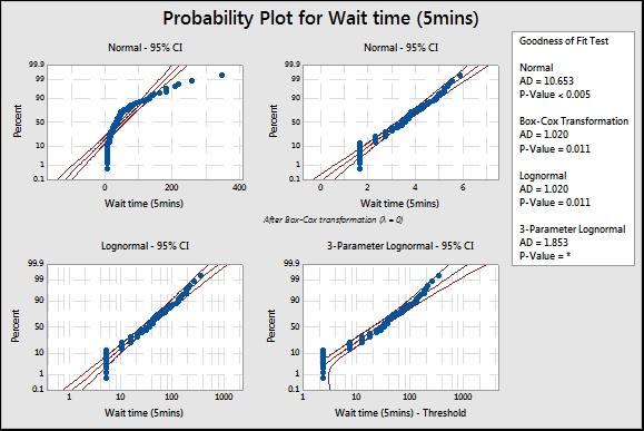
- All available P-values will be below 0.05, indicating that we can prove that none of those distributions fit those results. Instead, find the closest fits visually.
The ID plots will show P-values as below 0.05 for all distributions. The shape of the distributions also shows discrete intervals on most of the charts. In the preceding screenshot, you will notice the straight lines of the data points. The gaps and dots aligned are for the five-minute intervals. There is a large initial amount of data at five minutes, then a gap with no observations until the 10 minute result. The reason for not fitting any distribution is due to the data being discrete. Wait times really do not have exact five-minute gaps, but are an artifact of the measurement system.
In this recipe, we can still find the closest fit to the distribution graphically. As we know, the data has been split into discrete measurements and the actual times will really be from a continuous scale.
The lognormal distribution still provides a reasonable fit visually. Compare this to the result in the Capability analysis for nonnormal distributions recipe when using the one-minute interval data. In this case, we will analyze the data as a lognormal distribution. Run the five-minute interval column as a nonnormal capability analysis, follow the instructions for the earlier recipe, and substitute the five-minute interval data.
It is useful to compare the results either by using columns to see the effect that the discrete nature of the five-minute intervals has on the results. They will generate similar capability figures.
Examples of other data that may not fit a distribution include unstable processes, where the data exhibits shifts in the mean or variance, or other special causes. The results could be declared as not normal because the tails of the data show too many results or because outliers make the data not normal. Ideally, we would want to find the reason behind the unstable process rather than trying to find a distribution or transformation to use.
Another common set of data are measurement systems that do not report values below a certain number. Typically, we might see these types of measurements on recording amount or size of particles as a measure of contamination. The measurement device reports all values below a threshold as 0. The actual results are too small to resolve, and we do not know the true value for any figure recorded as zero. It could be zero or any value in the intervals from zero to 0.02. Recording the figures at zero creates a dataset with a gap and some start point, say 0.02.
As the actual value is unknown, rather than reporting the value as zero, data from this sort of measurement system can be reported as missing below the threshold of resolution. Alternatively, the zero values can be adjusted by adding a random value. Find the variation of the measurement device from a Gage study. Then generate random values with a mean of zero and the standard deviation of the measurement device. Add these values to the zeroes to generate a pseudo data point. Any negative values should be left as zero.