
Box-Cox transformations are used to transform a dataset that is not normally distributed. The transformed data is then fitted to a normal distribution and used to find a value for the capability of the process.
Nonnormal distributions in continuous data are typically associated with some form of boundary condition. Limits restrict the distribution in one direction. Good scenarios are where we have the boundary at 0. An example may include a measure of particle contamination in a packaging. The ultimate goal for medical devices would be to achieve zero particles; negative particle counts are not possible, and the closer we get to achieving the goal of zero, the more skewed our data can become.
Process times, again, are restricted to the 0 boundary; for example, we could study telephone answer times at a call centre. The time taken for an operator to pick up a call that is coming through to their phone cannot be negative; the phone must ring for them to answer the call.
We will use the example from the previous recipe for nonnormal distribution. The data is for patient waiting times at an accident and emergency ward. Patients should wait no more than 240 minutes before being seen by a doctor.
In the previous example, we used a distribution ID plot to find a distribution to fit to the data. Just like the lognormal distribution, the Box-Cox transformation also provided a reasonable fit.
Here, we will check the fit using the Box-Cox transformation under control charts before analyzing the capability with the normal distribution tools.
The following steps will check to see if the Box-Cox transformation will work on our data and then use the Capability Analysis tool's normal distribution with the transformation:
- Open the worksheet
Wait time.mtwby using Open Worksheet from the File menu. - Navigate to Stat | Control charts and select Box-Cox Transformation.
- Enter the column
Wait time (1Mins)in the section under the drop-down list and select All observations for a chart are in one column in the list. - Enter Subgroup sizes as
1. - Click on OK.
- The Box-Cox results indicate the use of Lambda for the transformation of 0. To use this with the capability analysis, navigate to Stat | Quality Tools | Capability Analysis and select Normal.
- Enter
Wait time (1 Mins)in the single column field and1in the Subgroup size. - Enter
240in the Upper spec field. - Click on the Transform button and select the Box-Cox power transformation radio button.
- Click on OK; then click on the button Options. Check the box Include confidence intervals. Change the Display section to percents.
- Click on OK in each dialog box.
The use of the Box-Cox Transformation tool in steps 1 to 4 is not necessary to run the capability. By using the distribution ID plots as in the previous recipe, we will see that the Box-Cox transformation will work on our results. The Box-Cox Transformation tool can show us the potential range of Lambda and can be used to store the transformed results back into the worksheet. The following screenshot shows the range of Lambda that would work for this data:
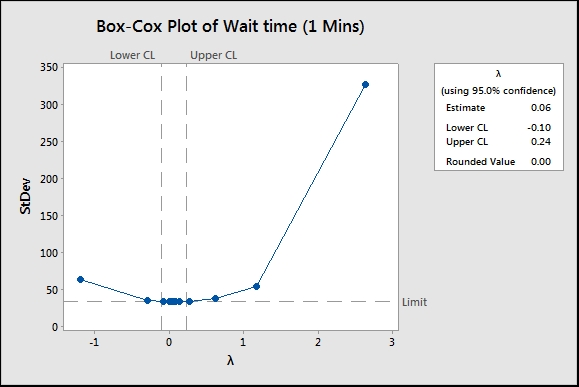
Box-Cox transformations are simple power transforms. The response Y is transformed by the function ![]() . When Lambda is 0, we use the natural log of the data. While the Box-Cox transformation used in steps 1 to 4 calculates an estimate for the Lambda value of 0.06, Minitab will work from a convenient rounded value, hence the value is 0.
. When Lambda is 0, we use the natural log of the data. While the Box-Cox transformation used in steps 1 to 4 calculates an estimate for the Lambda value of 0.06, Minitab will work from a convenient rounded value, hence the value is 0.
By transforming the times and the specification, this allows a fit for the normal distribution and a calculation of Cpk.
While choosing to transform the data within the Capability Analysis dialog box, we can specify the value of Lambda to use or let Minitab pick the best value itself. Minitab will use the rounded value when it picks the best value.
The Ppk value for the transformed results is 0.65. This is a slightly different result as compared to the previous recipe using the lognormal data. This is because we use the calculation of Cpk from a normal distribution here. The nonnormal capability uses an approximation based on the ISO method. Both the overall performance figures will be the same no matter what method is used to calculate capability.
The Assistant tool can also transform the data with a Box-Cox transformation. If the data is not normally distributed, the assistant will check the transformation and prompt us to ask if we would want to transform the results if it is possible. Note that we should not transform the data just because it is possible to; we should first investigate the cause of the data being nonnormal.