
Nonlinear regression tools give us the ability to specify an expectation function that goes beyond the Linear, Quadratic, or Cubic models. Applications of nonlinear regression are present where the Linear models fail to fit very well. Models for exponential growth and decay rates are good examples, where the nonlinear tools will provide a better fit to the data. The use of nonlinear regression tools is more complicated than the Linear models, and initial estimates of the coefficients must be provided.
Here we will use the data from the Oxford weather station to define our own expectation function, set the initial parameters of the function, and find the parameters of the coefficients. We will concentrate on the results from 2000 onwards, hence the initial steps will be to subset the worksheet.
From these results, we will define a regression model to predict the mean maximum monthly temperature from the month of the year.
The data for this example can be found on the Met Office website at the following link:
http://www.metoffice.gov.uk/climate/uk/stationdata/oxforddata.txt
Follow steps 1 to 12 from the Generating a paneled boxplot recipe in Chapter 2, Tables and Graphs, to import the results.
The data is also made available in the Oxford data.txt files; this preserves the format from the website. Also, the Oxford weather (Cleaned).MTW Minitab file is correctly imported into Minitab for us.
The following steps will create a subset of the worksheet using just the data from 2000 onwards. Then, we will use a Sine function to fit the mean maximum temperature by month:
- First, we will subset the data; use the Data menu and Subset Worksheet….
- Enter the name of the new worksheet as
Year 2000 onwards. - Select the Condition… button and enter the condition as
'Year' >= 2000. - Click on OK in each dialog box to create the new worksheet.
- To view the shape of the results, we will use a time series plot. Go to Graph and then select Time Series Plot….
- Select the Simple time series.
- Enter the column for mean maximum temperature in the Series: section.
- Click on the Time/Scale… button.
- Select the Stamp option and then select month and year as the stamp columns, as shown in the following screenshot:

- Click on OK in each dialog box.
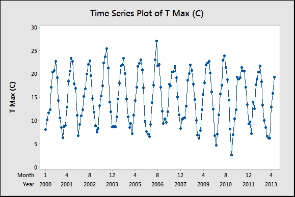
- The results should generate a regular pattern as shown in the following screenshot:
Note
Gaps in the chart will correspond to estimated temperatures. The table on the Met Office website marks these as values with a * symbol at the end. For example, 13.6* is an estimated temperature. Minitab will replace these values with a * symbol for the missing data when copying into the worksheet. These values can be corrected manually.
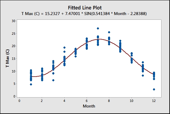
- We need to estimate an expectation function for temperature. The results follow a sinusoidal repeating pattern, with a range from minimum to maximum of roughly 20 degrees. The frequency of the Sine wave is every 12 months, with a mean value of roughly 15 degrees.
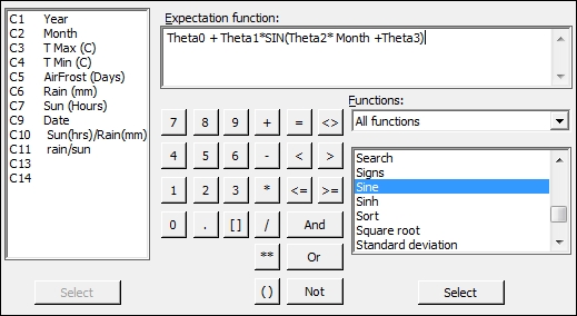
- A suitable form for the expectation function would be Mean + Magnitude *Sine(months). This can be written as follows:
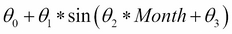
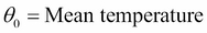
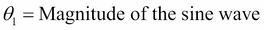
The respective parameters are explained as follows:

- To fit the model, navigate to Stat | Regression and select Non Linear Regression.
- In the Response: section, enter
TMaxfor mean maximum temperature. - Click on the Use Calculator… button to specify your expectation function.
- Enter values in the Expectation function: section, as shown in the following screenshot:
- Click on OK and then select the Parameters… button.
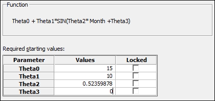
- Set the parameters with the following values as the starting points of the coefficients. Theta0 corresponds roughly to the mean temperature of 15 degrees. Theta1 is placed roughly at the magnitude of the wave at 10 degrees. Theta2 becomes 2*Pi/12 and Theta3 will be the start position of the sine wave that can be estimated at 0, as shown in the following screenshot:
- Click on OK and select the Options… button. Change Algorithm to Levenberg-Marquardt.
- Click on OK and select the Graphs… button.
- To check the assumptions of running the regression, select the Four in one residuals and click on OK in each dialog box.
Theta is traditionally used as our coefficient in nonlinear regression rather than beta, although it does not matter what name is used for the coefficients. Any text that is not recognized as a function, a column, or a constant is defined as a coefficient.
With the nonlinear regression, finding coefficients is not as simple as linear regression. We have to start with an estimate for the values of the coefficients. These starting points are then searched around with either the Gauss-Newton or Levenberg-Marquardt algorithms. Options within the main dialog box allow us to choose between the two search algorithms and specify the maximum number of iterations to find a solution.
If we are very wrong with the initial estimates, then the search algorithms may fail to converge on a solution. The session window will indicate whether this has happened. We could then expand the number of iterations, change the search algorithm, or recheck the estimates of the coefficients.
We have set the coefficients in this example as the mean temperature for Theta0; Theta1 is defined by the range/2 and Theta2 becomes 2*Pi/12; they give us the full number of radians in 12 months. Theta3 is defined as the offset to start the Sine function. Its parameters can be locked to fix the values of Theta. In this example, we may wish to lock Theta2 to 2*Pi/12.
Nonlinear regression has the same assumptions for the residuals and we should check the residuals for normality, equal variance, and independence over time.
This tool also contains a catalogue of predefined functions. We could select a number of these based on our knowledge of the process being studied or by the shape of the function.
As we define our own functions, these are saved within the catalogue as well. They are saved within the drop down under My functions. They can also be renamed and given a category.
With the study here, we looked at the relationship of month and temperature for the results after 2000. We could run the same study for all data from 1853 onwards. When running these results, try looking at the residual plots and see if there is anything unusual.
The benefit of the nonlinear regression tools is their ability to fit models where the standard Linear models do not quite work. Linear models also refer to Quadratic or Cubic models, which can be slightly confusing.
We could compare the results of this nonlinear regression using the Sine function to fit the month to a Quadratic model. We would obtain a result that seems to fit reasonably well; you should notice that around July and August and towards January and December, the data deviates appreciably from the fitted quadratic. The use of residual plots will reveal that the residuals versus fits still has a curved pattern, indicating poor fits across the line.
The use of the Sine function gives us a closer-fitting model over the results and a better predictive model. The simple sine function doesn't account for other random weather patterns, but still keeps a good fit for expected temperatures by month. The inclusion of terms to fit to trends over years or other predictors can help reveal more structure in the results.
A trend component can be added by including ![]() .
.
If we analyze this data using General Linear Model (GLM) or a one-way ANOVA, we will obtain a similar result. GLM will find the mean response for each month, rather than the equation obtained here.