
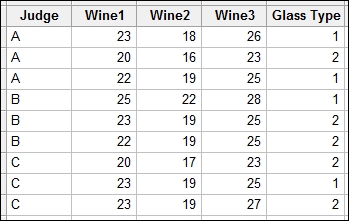
These studies use repeated measurements on a subject. Typically, they are used to assess the change over time, or the same observation under different conditions. In this recipe, the results of a blind wine tasting are studied. Three types of wine are tested by three judges; a third factor is included for the type of glass the wine is being tested in. The score is accumulated across several responses and the maximum score is 40.
We will stack the data first before using the general linear model to study the effect of Judge, Wine, and Glass type on the score. The Judge factor can be considered a random factor in the design. Wine and Glass become our fixed factors.
We will use a decision level of 0.05 for the p-value.
The following steps will stack the data in one column before using the general linear model. We then reduce the model by removing the terms by hierarchy and p-value:
- Navigate to Data | Stack and click on Blocks of Columns.
- Enter the columns in the dialog box as shown in the following screenshot. Uncheck the Use variable names in subscript column option.
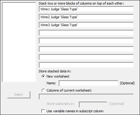
- Click on Ok to create the new worksheet.
- Name the new columns as
Wine,Score,Judge,Glass type. - Navigate to Stat | ANOVA | General Linear Model and click on Fit General Linear Model.
- Enter
Scorein the Responses: field. - In the Factors: field, enter
Wine Judge 'Glass type'. - Click on the Random/Nest… button and in the section for Factor type:, change Judge to Random.
- Click on OK and click on the Model… button.
- Highlight all three factors in the Factors and covariates: section and change Interactions through order: to 3. Then click on the Add button to add all two-way interactions and the three-way interaction to the model terms. Click on OK in each dialog box to run the analysis.
- Check the p-value of the three-way interaction. As this is above 0.05, press Ctrl + E to return to the General linear Model tool.
- Click on the Model… button and double-click on the three-way interaction in the Terms in the model: section to remove it from the study. Click on OK in each dialog to rerun the study.
- Return to the session window and check the results. Check the interactions for significance. Look for p-values less than 0.05; press Ctrl + E to return to the last dialog box.
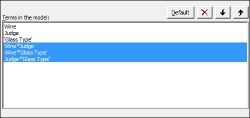
- As all two-way interactions are not significant, remove these by clicking on the Model… button. Highlight the two-way interactions as shown and click on the red X to remove these from the model. Click on OK in each dialog to rerun the study.
- Return to the session window and check the main effects for their significance. Use the decision level of 0.05 for the p-value.
- As all the terms are significant, press Ctrl + E to return to the last dialog and click on the Graphs… button. Select the Four in one residual plots. Click on OK in each dialog.
- To run comparisons of the wines on each other, navigate to Stat | ANOVA | General Linear Model and click on Comparisons. Double-click on Wine in the list under Choose terms for comparisons:.
Wineshould now be noted withCto indicate that this is selected. - Click on the Results… button and check the Tests and confidence intervals box.
- Click on OK in each dialog to generate the Tukey pairwise comparisons.
- To generate factor plots, navigate to Stat | ANOVA | General Linear Model and click on Factorials Plot.
- Click on OK to generate the main effects plots.
Judge is identified as a random factor as it is a random selection of Judge from a population of Wine tasters. The Wine column is a fixed factor as we wish to assess which wine has the greatest or lowest score. The glass type in the trial forms a fixed factor because we want to know how the glass type affects the score.
The section within the Fit General Linear Model tool for Random/Nest… allows us to identify factors as random, fixed, or nesting in the model. The Model… section gives us the ability to quickly add interaction terms to a study.
When entering columns, they can be typed in by name or column number, double-clicked to move across, or highlighted and then moved across by clicking on Select. If we are typing the names of the columns, we must use ' ' to identify any column name with spaces or special characters, a in 'Glass type'. Double-clicking or selecting columns into the model will automatically place single quotes where appropriate.
We specified a pairwise comparison of the wine results. Without changing the options, we obtain a grouping information table. This identifies the comparison levels by placing them into separate letter groups. This is generated for the selected comparison method. By selecting the option for Tests and confidence intervals, we output the results of the comparison as tables of t-values and p-values.
The interval plot for comparisons shows us the 95 percent confidence intervals for the differences between each pair of groups. Here, we should see that as all wine differences do not overlap the zero; we can prove a difference in score by wine.
The interval plot shows comparisons between pairs of wines. The x-axis displays the differences between the means of each pair of wines. A line at 0 is drawn to indicate 0 differences. Wine2 to Wine1 for instance shows a mean difference of -3.66 and a 95 percent confidence interval of -4.9 to -2.4. A confidence interval that crosses the zero line would indicate that there could be no difference between the means of that pair. Here none of the confidence intervals cross the zero line and all wines can be proved to be different to each other.