
In the previous recipes, we used normal distribution to estimate capability. When data is not distributed normally, the normal distribution will incorrectly estimate the amount of the results that we find outside of the specifications, and it makes the calculation of the capability inaccurate. Here, we will look to find an appropriate nonnormal distribution or transformation to fit to the data.
It is vital to indicate that before looking at transformations or nonnormal distributions, we must understand the process that we are investigating. We must consider the reasons for the data not being normal. An unstable process can fail the normality test because the mean or variation is moving over time. There may be trends or process shifts. With this data, we should investigate the issues of the unstable process before using transformations as a fix.
Other issues may be that we have several distributions within the block of data. Different machines produce the parts at different means, each machine makes items with a normal distribution, but combined together, we get a bimodal or multimodal distribution.
Measurement systems can also cause nonnormal data. If the measurement device is not accurate across the whole measurement range, a linearity problem may cause kurtosis. Resolution problems may mean that the results come from a discrete scale instead of a continuous scale.
Even a human error or intervention can cause data that is not normal. Specifications and deadlines can drive operators to behavior that places results just inside specification.
Lastly, if we are using an alpha risk of 0.05— the decision for the P-value—then there is still a 5 percent chance that normally distributed continuous data may fail the normality test just through random variation.
There should be a physical reason why our data follows a given distribution, and we would want to satisfy ourselves that the process is stable, the measurement system is verified, and that we have a single distribution. Finally, we understand why such data may not follow a normal distribution before we really look for the distribution that it does follow.
A good example of nonnormal distributions would be the process times. These typically follow a lognormal or a similar distribution due to there being a boundary at 0 time. To fit a nonnormal distribution, we will look at the waiting time experienced at an accident and emergency ward by all the patients across a day. The data set contains two columns of wait times reported at 1-minute intervals, and the same wait times reported at 5-minute intervals. The goal is that patients arriving at the A&E unit should be seen by a doctor within four hours (240 minutes).
We will initially use Distribution ID plots for the reported 1-minute wait times to find a distribution that fits the data. Then, we use capability analysis with the appropriate distribution and an upper specification limit of 240 minutes. See the example at the end of this chapter where we use the same data reported to the nearest 5-minute interval.
The following steps will identify a distribution that fits the wait time data before using a capability analysis with a lognormal distribution:
- Go to the File menu and click on Open Worksheet.
- Open the worksheet
Wait time.mtw. - Navigate to Stat | Quality tools | Individual Distribution Identification.
- Enter the
Wait time (1 Mins)column in the Single column field and the Subgroup size as1, as shown in the following screenshot: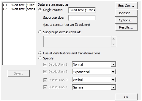
- Click on OK to generate the ID plots.
- Scan through each page, looking at the closeness of the fitted data looking graphically, the AD scores, and P-values for each distribution. An example of a distribution is shown in the following screenshot:
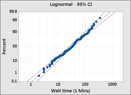
- We will use the lognormal distribution, as the data seems to fit the distribution. The Anderson-Darling test has low values and a P-value greater than 0.05.
- Navigate to Stat | Quality Tools | Capability Analysis and select Nonnormal.
- Insert the column
Wait time (1Mins)into the section Single column. - From the section Fit Distribution, select Lognormal.
- In Upper spec field, enter
240. - Select Options.
- In the Display section, select Percents.
- Click on OK in each dialog box.
The distribution ID plot generates probability plots for 14 different distributions and two transformations to find a fit to the data. We will use a visual inspection of the probability plots to identify which distributions give us a close fit to our results. Each probability plot will also run the Anderson-Darling statistics and generate a P-value.
Goodness of fit tests are generated in the session window. This allows a quick comparison across all the options. For the results here, we can see that several of the possible distributions may work for the wait times.
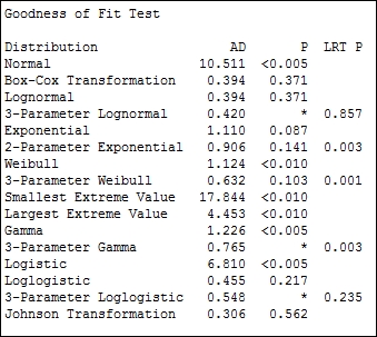
Some of the 3-parameter distributions do not have a P-value calculated; it can not be calculated easily and will show a missing value. In such instances, the LRT P value generated by the likelihood ratio test is a good test to use.
LRT P is generated for the 3- or 2-parameter extensions to a distribution. For example, the Weibull distribution with a threshold as the third parameter. LRT P tests the likelihood of whether the 3-parameter Weibull fits better than the standard Weibull distribution. In the above results, we can see that the 3-parameter Weibull has an LRT P of less than 0.05 and will give a different fit compared to the Weibull test.
The aim is to find the distribution to fit to the population. We should also consider what distribution is expected to fit the distribution. As we are dealing with times in this example, we can expect that the population of wait times will follow a lognormal distribution. As the P-value for the lognormal is above 0.05, we cannot prove that it does not fit this distribution. When selecting a distribution, we would want to preferentially use the expected or historically observed distribution. In practice, distributions that fit in similar ways will give similar results.
We used the nonnormal capability analysis here to use the lognormal distribution. If we had wanted to apply a transformation to the data, we would use the normal capability analysis. See the Box-Cox and Johnson transformation subjects.
There is no calculation of within group variation with nonnormal distributions. Due of this, only Ppk for the overall capability is calculated. Within capability is only calculated for a normal distribution. To obtain an estimate of Cpk, we would need to use a Box-Cox transformation. Also, without Cpk and within variation, there is no requirement to enter the subgroup size for the nonnormal capability.
We could run a similar sixpack on nonnormal capability, as illustrated in the normal capability sixpack. This will require a subgroup size only to be used with the control charts.
As we only have an upper specification, we will only obtain Ppu, the capability to the upper specification. There will be no estimate of Pp.
Strictly speaking, capability is calculated as the number of standard deviations to a specification from the mean divided by 3. As the data is not normally distributed, this is not an accurate technique to use. There are two methods that Minitab can use to calculate capability for nonnormal data.
The ISO method uses the distance from the 50th percentile to the upper or lower specification divided by the distance from the 50th percentile to the 99.865th or 0.135th percentile.
For the example here with only an upper specification, we have the Ppk calculated from the PpU by using the formula
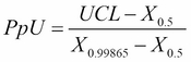
Here, X0.5 refers to the 50th percentile and X0.99865 refers to the 99.865th percentile.
This formula uses the equivalent positions of the +/-3 standard deviation point of a normal distribution. It does not always give the same capability indices like a transformed data set using the normal capability formula. The proportion outside the specification will be similar throughout. See the Box-Cox transformation in Minitab for more information.
An alternative is to use the Minitab method. It can be selected from the options for Minitab under the Tools menu, which is in Quality tools under Control Charts.
This method finds the proportion of the distribution outside the specification. Then, it finds the equivalent position on a standard normal distribution. This equivalent position for Z is divided by 3 to give the capability.
We should also look at the data for waiting times that has been recorded to the nearest five minutes. When used with the distribution ID plots, notice what happens to our results. For more on this, see the datasets that do not transform or fit any distribution.