
In the random effects model, both factors are declared as random factors. This recipe looks at a study on taste from a panel of professional taste testers. Different batches of a food product are tested to check the consistency of taste. Each appraiser tastes each batch twice. This way we can observe the consistency of scores from within the appraiser.
As the product is a selection of batches from a much larger population of batches, the samples represent a random selection from all product batches. The taste testers are a sample of appraisers from a group of tasters, representing a random selection as well; we will use the appraiser as a random factor to represent the variation across appraisers.
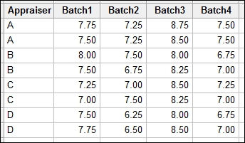
The scores are a mean figure from four attributes: taste, aroma, texture, and appearance.
The data will be provided later to type into Minitab; for ease of entry, it is set out as a table. We will stack this into columns to run the general linear model with both factors defined as random factors.
The following steps will stack the data into a new worksheet. After renaming the stacked data, we will look at the effects of the batch and the appraiser on the taste scores using a general linear model:
- Navigate to Data | Stack and click on Blocks of Columns.
- Enter the columns into the dialog as shown in the following screenshot:
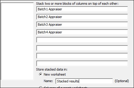
- Click on OK to create a new worksheet with the stacked data.
- Rename column 1 as
Batch, column 2 asScore, and column 3 asAppraiser. - Navigate to Stat | ANOVA and click on Fit General Linear Model.
- Enter
Scorein the Responses: field and in the Factors: field, enterBatch Appraiser. - Select the Random/Nest… button.
- Change Factor type: to Random for both the Batch and Appraiser columns, as shown in the following screenshot:
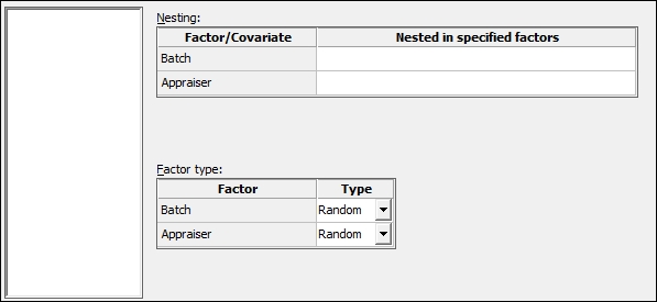
- Click on OK.
- Next, click on the Model… button.
- Highlight Batch and Appraiser in the Factors and covariates: section and then click on the Add button next to the Interactions through order: field. As shown in the following screenshot, add the interaction of
BatchandAppraiserto the model: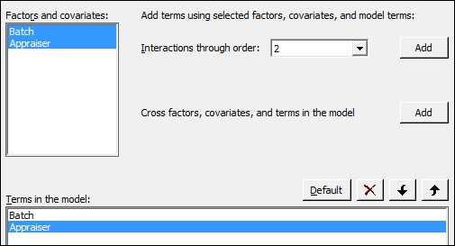
- Click on OK in each dialog box to run the analysis.
- Check the results in the session window. Use a decision level of 0.05 for the p-value.
- As the interaction between
BatchandAppraiseris significant, we will leave all terms in the model. To check the assumptions of using the general linear model, we will generate residual plots. Press Ctrl + E to return to the last dialog box. - Click on the Graphs button and select the Four in one option.
- Click on OK in each dialog box to run the study.
The random effects model from the general linear model will find the F-statistics for the factors of Batch and Appraiser from the following expression: ![]() . As both factors are random, the error for these terms is found from the interaction term.
. As both factors are random, the error for these terms is found from the interaction term.
To define the model that we are fitting, we enter all the factors into the factors section within Minitab, and any covariates would be entered into the separate covariate section. Then we use the Random/Nest… button to identify nesting and random factors in the design.
The Terms… button gives us the options to identify the terms to be included in the model. We select the factors from the Factors and covariates: section and then by selecting the Interactions through order: field, all interactions for the highlighted factors up to the stated order would be included.
For example, if we have the three factors A B C and the D covariate, we could highlight A and B and select interactions up through order 2 to include the A*B interaction. Alternatively, we could highlight A through D and select order 3 and then we could include the interactions AB AC AD BC BD CD and the three-way interactions.
Quadratic or cubic effects on covariates can be included in the Terms through order: option. Note that this will be available only when covariates are included in the model.
This change for Minitab v17 makes the inclusion and removal of terms much simpler than it previously was. When reducing a model, we only need to highlight the terms that would be removed from the model and click on the X button to remove them.
The data supplied here was provided in a tabular format. Instructions 1 to 3 stack the data to be used in the general linear model tools. If our data was provided in this format, then we could skip these steps.
The GLM is run first with all the terms included. We check the results of the p-values and if the interaction cannot be proved as significant, then we would remove this term. At this point, we would return to the GLM and remove the interaction from the study. Without any interactions in a study with random factors, then the F-statistic for the main effects returns to mean square divided by the mean square error.
Finally, when only the significant terms are left in the model, we include the residual plots in the response, so we can verify the assumptions of using the analysis of variance. With the results of this study, we should notice an odd effect on the probability plot of the residuals. This is because the results are very discrete in nature.
The general linear model tool in Minitab will fit the unrestricted form of the ANOVA. For the restricted model, use the balanced ANOVA and select the restricted model from options.
For more on random effects models, see, Applied Linear Statistical Models, Fourth Edition, by Neter, Kutner, Nachtsheim, and Wasserman, page 1005.
The GLM tools have changed a lot for Minitab v17. With the previous version of Minitab, the dialog box will follow the same setup as the balanced ANOVA tools. This has changed how we enter terms into the model and also how we define nested or random factors.
The Fit General Linear Model option also stores the model in the response column of the worksheet. When returning to the worksheet, there will be a green tick in the Score column to indicate that we have a model fitted to Score.
This model can be used to run multiple comparisons and generate plots based on predicted values of the model.
Users of previous versions of Minitab will also notice that the output of the GLM tools has been greatly expanded. The Results… button gives us a lot of control over the amount of output we can choose to display. Everything from the model summaries, regression equations, variance components, and much more can be expanded from here.
Other new options for GLM with Minitab v17 include the ability to standardize the covariates. We have five options to help standardize the covariates:
- Low and high levels standardized to -1, +1
- Subtract the mean and divide by the standard deviation
- Subtract the mean
- Divide by standard deviation
- Subtract by a value and divide by another specified value
- The Analyzing a balanced design recipe
- The Stacking blocks of columns at the same time recipe in Chapter 1, Worksheet, Data Management, and the Calculator
- The Using GLM for unbalanced designs recipe