
This recipe will look at studying a multiple regression on determining the sleep duration of mammals. The dataset is available at StatSci.org.
We will run the study with all predictors included for the initial model and then remove the terms in the model step-by-step. Our goal is to reduce the terms until only the significant ones are left. As this data does have a degree of correlation among the predictors, we will use matrix plots, correlation, and variance inflation factors to highlight the degree of multicollinearity.
We will initially produce the matrix plots and the correlation scores before moving on to the analysis of the regression.
After reducing the model to only significant terms, we will then produce the residual plots to gradually verify assumptions on the analysis.
The value of alpha for the decision level used here will be 0.05.
The data is available at the following link from StatSci.org:
http://www.statsci.org/data/general/sleep.html
The data is tab delimited and can be copied directly into the worksheet.
The following steps will run a regression that studies the sleep duration. We will produce a matrix plot and correlation scores to check for multicollinearity before using regression to gradually reduce the model until only the significant terms remain included:
- Go to the Graph menu and select Matrix Plot….
- From the selection, choose the Simple matrix plot.
- Enter the columns
BodyWt,BrainWt,TotalSleep,Lifespan,Gestation,Predation,Exposure, andDangeras Graph variables:. - Click on Matrix Options… and then select the option to display Lower left of Matrix Display.
- Click on OK in each dialog box to produce a matrix of scatterplots.
- Display the correlation scores by going to Stat, then Basic Statistics, and then Correlation….
- Enter the same columns as before into the Variables: section and click on OK to generate the correlation scores.
- Navigate to Stat | Regression | Regression… and select Fit Regression Model….
- Enter
TotalSleepas the column for Response. - In the section for Continuous predictors:, enter the columns for
BodyWt,BrainWt,Lifespan,Gestation,Predation,Exposure, andDanger. - Click on OK to run the regression.
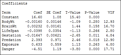
- Return to the session window and check the results for the regression. Check the terms for the highest P-value, as shown in the following screenshot:
- Press Ctrl+E to return to the last dialog box and remove the term with the highest P-value, BodyWt, from the Continuous predictors.
- Return to the session window and look for the term with the highest P-value.
- Repeat steps 12 to 14 until only the terms with a P-value below 0.05 are included.
- With only those terms included for the final results, go back to the Regression dialog box by pressing Ctrl+E and then go to the Graphs… button. Select the Normal plot of residuals and Residuals vs fits.
- Click on OK in each dialog box.
The model is reduced sequentially to minimize the problems of multicollinearity in the predictors. The reason for generating the matrix plots and correlation scores is to observe the relationships in the predictors that we have to be careful of. We should observe strong correlations between body weight and brain weight, predation and danger, exposure and danger, among others. We will find it difficult to isolate the effects of highly correlated predictors.
Variance inflation factors (VIF) in the output also identifies strong correlations between predictors. The variance inflation factor is a measure of how the variance of the coefficients is inflated by multicollinearity. High VIF scores can indicate that terms in the model are difficult to interpret. Predation and danger, as observed in the correlation scores and the matrix plots, will show a high VIF. Values of 1 will indicate no inflation of the variance and values above 5 will indicate high correlations. As such, we should be careful of any terms with high VIF scores such as predation and danger, as these are strongly correlated.
Residual plots for order of the data are not needed as the worksheet is ordered alphabetically. When our results do not appear to follow a logical order in the dataset, we should not run the versus order charts. The residual versus fits for this study may seem to indicate a degree of funneling, as shown the following screenshot:

Funneling is an indicator that the response does not possess equal variance across the fitted values and that we are observing heteroscedasticity.
The assumptions for a regression analysis include normally distributed residuals and homoscedasticity. When we are concerned about unequal variance in the residuals, a transformation of the response may be used. Here, a natural log of the sleep duration can be used to return the residuals to show equal variance.
The effect of unequal variance on the results can be to calculate coefficients and variance figures incorrectly. Transformations on the response can help find the values of the variance and coefficients with a better precision. However, we must be careful that we understand the reasons behind transformation of the data. Transformation of the data is not a technique to fix outliers or special causes in our results.
We can run a transformation on the response directly from the regression options. Minitab can be allowed to pick an optimal lambda for the transformation or it can be specified directly. Try running the same regression with the Box-Cox… options. You should obtain a similar model with transformed and untransformed data.
Interactions, Quadratic, and Cubic terms can be easily specified from within the Model… options of the Fit Regression Model… dialog box.
Predictors can be standardized as well. Standardizing the predictors can be a useful method to reduce multicollinearity between predictors. The Coding… options give us five methods to standardize predictors.
The Stepwise… options allow us to use a stepwise model fitting technique. Here, we can choose between stepwise, forward, or backward selection.
The session window is 93 characters wide by default. With large correlation tables or long column names in a study, this can cause a table to be presented across several lines, with the last columns spilling over into a new table.
The options for Minitab, found in the Tools menu, can expand the session window's width to 132 characters.